Missing data pattern summary statistics

• When the number of columns is small, we can use the md.pattern function in mice to get missing data counts of all combinations among columns

library(mice); 
md.pattern(pattern4, plot = FALSE)

##   A B C  
## 2 1 1 1 0
## 3 1 1 0 1
## 1 1 0 1 1
## 2 0 0 1 2
##   2 3 3 8

• When the number of columns is large, we can use the md.pairs function in mice to check the counts of each of the four pairwise missingness patterns (rr, rm, mr, and mm)

Inbound and outbound statistics: measure pairwise missing patterns

• Proportion of usable cases, i.e., inbound statistics for imputing variable \(Y_j\) from variable \(Y_k\): total cases where \(Y_j\) is missing but \(Y_k\) is observed over total missings in \(Y_j\) \[ I_{jk} = \frac{\sum_{i=1}^n (1 - r_{ij}) r_{ik}}{\sum_{i=1}^n (1 - r_{ij})} \]
  • When imputing \(X_j\), we can use this statistic to quickly identify which variables to use
• Outbound statistic measures how observed data in \(Y_j\) connect to the missing data in \(Y_k\) \[ O_{jk} = \frac{\sum_{i=1}^n r_{ij} (1 - r_{ik})}{\sum_{i=1}^n r_{ij}} \]

Different imputation strategies for different missing patterns

• Monotone data imputation

  • for monotone missing data pattern
  • imputations are created by a sequence of univariate methods

• Joint modeling (JM)

  • for general missing patterns,
  • imputations are created by multivariate models

• Fully conditional specification (FCS, aka chained equations)

  • for general missing patterns,
  • imputations are drawn from iterated conditional univarate models
  • Usually, FCS is found better than JM

• Block of variables, hybrid imputation between JM and FCS

Monotone data imputation

• A monotone missing pattern: the columns of \(Y\) can be ordered such that for any row, if \(Y_j\) is missing, then all columns to the right of \(Y_j\) are also missing

• Suppose the variables with missings are ordered as \(Y_1, Y_2, \ldots, Y_p\), and the variables without missings are denoted as \(X\). Then the monotone missing imputation is

  • Impute \(Y_1\) from \(X\)
  • Impute \(Y_2\) from \((Y_1, X)\)
  • …
  • Impute \(Y_p\) from \((Y_1, \ldots, Y_{p-1}, X)\)

Fully conditional sepcification (FCS): similar to Gibbs sampling

• FCS specifies the multivariate distribution \(p(Y, X, R\mid \theta)\) through a set of conditional densities \(p(Y_j \mid X, Y_{-j}, R, \phi_j)\)

• The conditional density is used to impute \(Y_j\) given \(X, Y_{-j}, R\) (including the most recent imputed values). \[\begin{align*} \dot{\phi}_j & \sim p(\phi_j \mid Y_j^\text{obs}, \dot{Y}_{-j}, R)\\ \dot{Y}_j & \sim p(Y_j^\text{mis}\mid Y_j^\text{obs}, \dot{Y}_{-j}, R, \phi_j) \end{align*}\]
  • We can use the univariate imputation method introduced in Chapter 3 as building blocks
• To initialize, we can impute from the marginal distributions
• One iteration consists of one cycle through all \(Y_j\). Total number of iterations \(M\) can often be low, e.g., 5, 10, or 20.

• For multiple imputation, perform this process in parallel for \(m\) times

Convergence of FCS (and in general of a Markov chain)

• Irreducible: the chain must be able to reach all interesting parts of the state space

  • Easy; users have large control over the interesting parts.

• Aperiodic: the chain should not oscillate between different states

  • A way to diagnose is to stop the chain at different points, and make sure stopping point does not affect statistical inferences

• Recurrence: all interesting parts can be reached infinitely often, at least from almost all starting points

  • May be diagnosed from traceplots

Compatibility

• Two conditional densities \(p(Y_1 \mid Y_2)\), \(p(Y_2 \mid Y_1)\) are compatible if
  • a joint distribution \(p(Y_1, Y_2)\) exists, and
  • it has \(p(Y_1 \mid Y_2)\) and \(p(Y_2 \mid Y_1)\) as its conditional densities

• FCS is only guaranteed to work if the conditionals are compatible

• The MICE algorithm (the FCS implemented in mice package) is ignorant of the non-existence of joint distribution, and imputes anyway.

  • Empirical evidence suggests the estimation results may be robust against violations of compatibility

Number of FCS iterations

• Why can the number of iterations in FCS be low (usually 5-20)?

  • The imputed data \(\dot{Y}_\text{mis}\) can have a considerable amount of random noise
  • Hence if the relations between the variables are not strong, the autocorrelation over iteration may be low, and thus convergence can be rapid

• Watch out for the following situations:

  • the correlations between \(Y_j\)’s are high
  • missing rates are high
  • constraints on parameters across different variables exist

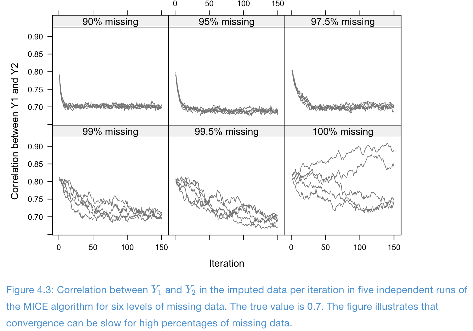
Example of slow convergence: design of simulation

• One completed covariate \(X\) and two incomplete variables \(Y_1, Y_2\)
• Data are draw from multivariate normals with correlations \[ \rho(X, Y_1) = \rho(X, Y_2) = 0.9, \quad \rho(Y_1, Y_2) = 0.7 \]
• Total sample size \(n=10000\), and completely observed cases \(\in \{1000, 500, 250, 100, 50, 0\}\)
• Imputation models are normal linear regressions (PMM)

Example of slow convergence: traceplots

• Missing problem with high correlation and high missing rates: convergence is poor

References

• Van Buuren, S. (2018). Flexible Imputation of Missing Data, 2nd Edition. CRC press.

  • https://stefvanbuuren.name/fimd/