For the pdf slides, click here
Introduction to Instrumental Variables
Unmeasured confounding
- Suppose there are unobserved variables \(U\) that affect both \(A\) and \(Y\), then \(U\) is an unmeasured confounding
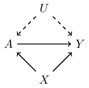
This violates ignorability assumption
Since we cannot control for the unobserved confounders \(U\) and average over its distribution, if using matching or IPTW methods, the estimates of causal effects is biased
Solution: instrumental variables
Instrumental variables
- Instrumental variables (IV): an alternative causal inference method that does not rely on the ignorability assumption
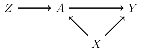
\(Z\) is an IV
- It affects treatment \(A\), but does not directly affect the outcome \(Y\)
- We can think of \(Z\) as encouragement (of treatement)
Example of an encouragement design
- \(A\): smoking during pregnancy (yes/no)
- \(Y\): birth weight
\(X\): mother’s age, weight, etc
- Concern: there could be unmeasured confounders
- Challenge: it is not ethical to randomly assign smoking
\(Z\): randomized to either received encouragement to stop smoking (\(Z=1\)) or receive usual care (\(Z=0\))
- Causal effect of encouragement, also called intent-to-treat (ITT) effect, may be of some interest \[E\left(Y^{Z=1}\right)-E\left(Y^{Z=0}\right)\]
- Focus of IV methods is still causal effect of the treatment \[E\left(Y^{A=1}\right)-E\left(Y^{A=0}\right)\]
IV is randomized
Like the previous smoking example, sometimes IV is randomly assigned as part of the study
Other times IV is believed to be randomized in nature (natural experiment). For example,
- Mendelian randomization (?)
- Quarter of birth
- Geographic distance to specialty care provider
Randomized trials with noncompliance
Randomized trials with noncompliance
- Setup
- \(Z\): randomization to treatment (1 treatment, 0 control)
- \(A\): treatment received, binary (1 treatment, 0 control)
- \(Y\): outcome
- Due to noncompliance, not everyone assigned treatment will actually receive the treatment, and vice verse (\(A \neq Z\))
- There can be confounding \(X\), like common causes affecting both treatment received \(A\) and the outcome \(Y\)
- It may be reasonable to assume that \(Z\) does not directly affect \(Y\)

Causal effect of assignment on receipt
Observed data: \((Z, A, Y)\)
Each subject has two potential values of treatment
- \(A^{Z=1} = A^1\): value of treatment if randomized to treatment
- \(A^{Z=0} = A^0\): value of treatment if randomized to control
- Average causal effect of treatment assignment on treatment received
\[E\left(A^1 - A^0\right)\]
- If perfect compliance, this would be \(1\)
- By randomization and consistency, this is estimable from the observed data \[ E\left(A^1\right) = E(A \mid Z=1), \quad E\left(A^0\right) = E(A \mid Z=0) \]
Causal effect of assignment on outcome
Average causal effect of treatment assignment on the outcome \[E\left(Y^{Z=1} - Y^{Z=0}\right)\]
- This is intention-to-treat effect
- If perfect compliance, this would be equal to the causal effect of treatment received
- By randomization and consistency, this is estimable from the observed data \[ E\left(Y^{Z=1}\right) = E(Y \mid Z=1), \quad E\left(Y^{Z=0}\right) = E(Y \mid Z=0) \]
Compliance classes
Subpopulations based on potential treatment
| \(A^0\) | \(A^1\) | Label |
|---|---|---|
| 0 | 0 | Never-takers |
| 0 | 1 | Compliers |
| 1 | 0 | Defiers |
| 0 | 0 | Always-takers |
- For never-takers and always-takers,
- Encouragement does not work
- Due to no variation in treatment received, we cannot learn anything about the effect of treatment in these two subpopulations
- For compliers, treatment received is randomized
- For defiers, treatment received is also randomized, but in the opposite way
Local average treatment effect
- We will focus on a local average treatment effect, i.e., the complier average causal effect (CACE)
\[\begin{align*} & E\left(Y^{Z=1} \mid A^0=0, A^1=1 \right) - E\left(Y^{Z=0} \mid A^0=0, A^1=1 \right)\\ = & E\left(Y^{Z=1} - Y^{Z=0} \mid \text{compliers} \right)\\ = & E\left(Y^{a=1} - Y^{a=0} \mid \text{compliers} \right) \end{align*}\]
- “Local”: this is a causal effect in a subpopulation
- No inference about defiers, always-takers, or never-takers
Instrumental variable assumptions
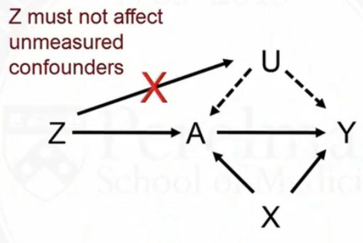
IV assumption 1: exclusion restriction
- \(Z\) is associated with the treatment \(A\)
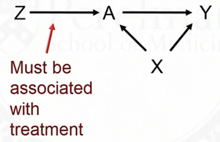
\(Z\) affects the outcome only through its effect on treatment
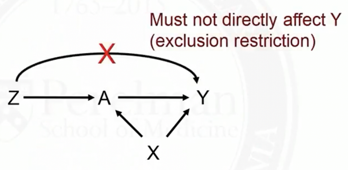
- \(Z\) cannot directly, or indirectly though its effect on \(U\), affect \(Y\)
Is the exclusion restriction assumption realistic?
If \(Z\) is a random treatment assignment, then the exclusion restriction assumption is met
- It should affect treatment received
- It should not affect the outcome or unmeasured confounders
However, it the subjects or clinicians are not blinded, knowledge of what they are assigned to could affect \(Y\) or \(U\)
We need to examine the exclusion restriction assumption carefully for any given study
IV assumption 2: monotonicity
Monotonicity assumption: there are no defiers
- No one consistently does the opposite of what they are told
- Probability of treatment should increase with more encouragement
With monotonicity,
| \(Z\) | \(A\) | \(A^0\) | \(A^1\) | Class |
|---|---|---|---|---|
| 0 | 0 | 0 | ? | Never-takers or compliers |
| 0 | 1 | 1 | 1 | Always-takers |
| 1 | 0 | 0 | 0 | Never-takers |
| 1 | 1 | ? | 1 | Always-takers or compliers |
Estimate Causal Effects with Instrumental Variables
Estimate CACE: 1. rewrite the ITT effect
Due to randomization, we can identify the ITT effect \[ E\left( Y^{z=1} - Y^{z=0} \right) = E(Y\mid Z=1) - E(Y\mid Z=0) \]
Expand the first term in the above ITT effect \[\begin{align*} E(Y\mid Z=1) = & E(Y\mid Z=1, \text{always takers})P(\text{always takers}\mid Z=1)\\ & + E(Y\mid Z=1, \text{never takers})P(\text{never takers}\mid Z=1)\\ & + E(Y\mid Z=1, \text{compliers})P(\text{compliers}\mid Z=1) \end{align*}\]
- Note 1: among always takers and never takes, \(Z\) does nothing
- \(E(Y\mid Z=1, \text{always takers}) = E(Y\mid \text{always takers}), \quad \text{etc.}\)
- Note 2: by randomization,
- \(P(\text{always takers}\mid Z=1) = P(\text{always takers}), \quad \text{etc.}\)
Estimate CACE: 1. rewrite the ITT effect, cont.
Therefore, the first term in the ITT effect is \[\begin{align*} E(Y\mid Z=1)=& E(Y\mid\text{always takers})P(\text{always takers})\\ & + E(Y\mid \text{never takers})P(\text{never takers})\\ & + E(Y\mid Z=1, \text{compliers})P(\text{compliers}) \end{align*}\]
Similarly, the second term is \[\begin{align*} E(Y\mid Z=0)=& E(Y\mid\text{always takers})P(\text{always takers})\\ & + E(Y\mid \text{never takers})P(\text{never takers})\\ & + E(Y\mid Z=0, \text{compliers})P(\text{compliers}) \end{align*}\]
Their difference is \[\begin{align*} & E(Y\mid Z=1) - E(Y\mid Z=0)\\ = & \left[E(Y\mid Z=1, \text{compliers})- E(Y\mid Z=0, \text{compliers})\right]P(\text{compliers}) \end{align*}\]
Estimate CACE: 2. compute proportion of compliers
Thus, the relationship between CACE and ITT effect is \[ \text{CACE} = \frac{E(Y\mid Z=1) - E(Y\mid Z=0)}{P(\text{compliers})} \]
To compute \(P(\text{compliers})\), note that
- \(E(A\mid Z=1)\): proportion of always takers plus compliers
- \(E(A\mid Z=0)\): proportion of always takers
Thus the difference is \[ P(\text{compliers}) = E(A\mid Z=1) - E(A\mid Z=0) \]
Estimate CACE: final formula
\[ \text{CACE} = \frac{E(Y\mid Z=1) - E(Y\mid Z=0)} {E(A\mid Z=1) - E(A\mid Z=0)} \]
Numerator: ITT, causal effect of treatment assignment on the outcome
- Denominator: causal effect of treatment assignment on the treatment received
- Denominator is between 0 and 1. Thus, CACE \(\geq\) ITT
- ITT is underestimate of CACE, because some people assigned to treatment did not take it
If perfect compliance, CACE \(=\) ITT
IVs in observational studies
IVs in observational studies
IVs can also be used in observational (non-randomized) studies
- \(Z\): instrument
- \(A\): treatment
- \(Y\): outcome
- \(X\): covariates
- \(Z\) can be thought of as encouragement
- If binary, just encouragement yes or no
- If continuous, a ‘dose’ of encouragement
\(Z\) can be thought of as randomizers in natural experiments
- The key challenge: think of a variable that affects \(Y\) only through \(A\)
- Only the assumption \(Z\) affecting \(A\) can be checked with data
- The validity of the exclusion restriction assumption rely on subject matter knowledge
Natural experiment example 1: calendar time as IV
Rationale: sometimes treatment preferences change over a short period of time
\(A\): drug A vs drug B
\(Z\): early time period (drug A is encouraged) vs late time period (drug B is encouraged)
\(Y\): BMI
Natural experiment example 2: distance as IV
Rationale: shorter distance to NICU is an encouragement
\(A\): delivery at high level NICU vs regular hospital
\(Z\): differential travel time from nearest high level NICU to nearest regular hospital
\(Y\): mortality
More examples of natural experiments
Mendelian randomization: some genetic variant is associate with some behavior (e.g., alcohol use) but is assumed to not be associated with outcome of interest
Provider preference: use treatment prescribed to previous patients as an IV for current patient
Quarter of birth: to study causal effect of years in school on income
Two stage least squares
Ordinary least squares (OLS) fails if there is confounding
- In OLS, one important assumption is that the covariate \(A\) is independent with residuals \(\epsilon\)
\[ Y_i = \beta_0 + A_i \beta_1 + \epsilon_i \]
However, if there is confounding, \(A\) and \(\epsilon\) are correlated. So OLS fails.
Two stage least squares can estimate causal effect in the instrumental variables (IV) setting
Two stage least squares (2SLS)
- Stage 1: regress \(A\) on \(Z\)
\[
A_i = \alpha_0 + Z_i \alpha_1 + e_i
\]
- By randomization, \(Z\) and \(e\) are independent
- Obtain the predicted value of \(A\) given \(Z\) for each subject
\[
\hat{A}_i = \hat{\alpha}_0 + Z_i \hat{\alpha}_1
\]
- \(\hat{A}\) is projection of \(A\) onto the space spanned by \(Z\)
- Stage 2: regress \(Y\) on \(\hat{A}\)
\[
Y_i = \beta_0 + \hat{A}_i \beta_1 + \epsilon_i
\]
- By exclusion restriction, \(Z\) is independent of \(Y\) given \(A\)
Interpretation of \(\beta_1\) in 2SLS: the causal effect
Consider the case where both \(Z\) and \(A\) are binary \[ \beta_1 = E\left(Y \mid \hat{A}=1 \right) - E\left(Y \mid \hat{A}=0 \right) \]
There are two values of \(\hat{A}\) in the 2nd stage model, \(\hat{\alpha}_0\) and \(\hat{\alpha}_0 + \hat{\alpha}_1\)
- When we go from \(Z=0\) to \(Z=1\), what we observe is going from \(\hat{\alpha}_0\) to \(\hat{\alpha}_0 + \hat{\alpha}_1\)
- We observe a mean difference of \(\hat{E}(Y\mid Z=1) - \hat{E}(Y\mid Z=0)\) with a \(\hat{\alpha}_1\) unit change in \(\hat{A}\)
Thus, we should observe a mean difference of \(\frac{\hat{E}(Y\mid Z=1) - \hat{E}(Y\mid Z=0)}{\hat{\alpha}_1}\) with \(1\) unit change in \(\hat{A}\)
The 2SLS estimator is a consistent estimator of the CACE \[ \beta_1 = \text{CACE} = \frac{\hat{E}(Y\mid Z=1) - \hat{E}(Y\mid Z=0)}{\hat{E}(A\mid Z=1) - \hat{E}(A\mid Z=0)} \]
More general 2SLS
2SLS can be used
- with covariates \(X\), and
- for non-binary data (e.g, a continuous instrument)
Stage 1: regression \(A\) on \(Z\) and covariates \(X\)
- and obtain the fitted values \(\hat{A}\)
Stage 2: regress \(Y\) on \(\hat{A}\) and \(X\)
- Coefficient of \(\hat{A}\) is the causal effect
Sensitivity analysis and weak instruments
Sensitivity analysis
Sensitivity analysis method studies when each of the IV assumption (partly) fails
- Exclusion restriction: if \(Z\) does affect \(Y\) by an amount \(p\), would my conclusion change? Vary \(p\)
- Monotonically: if the proportion of defiers was \(\pi\), would my conclusion change?
Strength of IVs
Depend on how well an IV predicts treatment received, we can class it as a strong instrument or a weak instrument
For a weak instrument, encouragement barely increases the probability of treatment
Measure the strength of an instrument: estimate the proportion of compliers \[ E(A \mid Z=1) - E(A \mid Z=0) \]
- Alternatively, we can just use the observed proportions of treated subjects for \(Z=1\) and for \(Z=0\)
Problems of weak instruments
Suppose only 1% of the population are compliers
Then only 1% of the samples have useful information about the treatment effect
- This leads to large variance estimates, i.e., estimate of causal effect is unstable
- The confidence intervals can be too wide to be useful
References
Coursera class: “A Crash Course on Causality: Inferring Causal Effects from Observational Data”, by Jason A. Roy (University of Pennsylvania)