For the pdf slides, click here

When data is not stationary

Implication of not stationary: sample ACF or sample PACF do not rapidly decrease to zero as lag increases
What shall we do?
- Differencing, then fit an ARMA $\to$ ARIMA
- Transformation, then fit an ARMA
- Seasonal model $\to$ SARIMA

A non-stationary exmaple: Dow Jones utilities index data

library(itsmr); ## Load the ITSM-R package
par(mfrow = c(1, 3));
plot.ts(dowj, main = 'Raw data'); 
acf(dowj); pacf(dowj);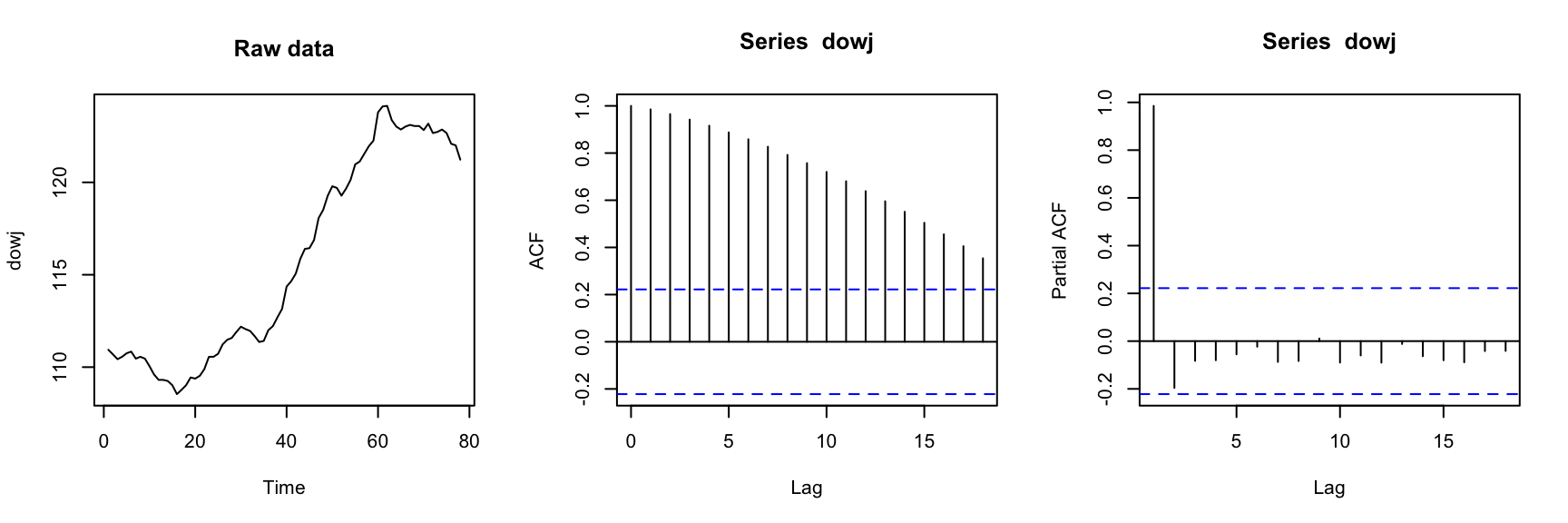

After differencing

par(mfrow = c(1, 3));
dowj_diff = dowj[-length(dowj)] - dowj[-1];
plot.ts(dowj_diff, main = 'Data after differencing'); 
acf(dowj_diff); pacf(dowj_diff);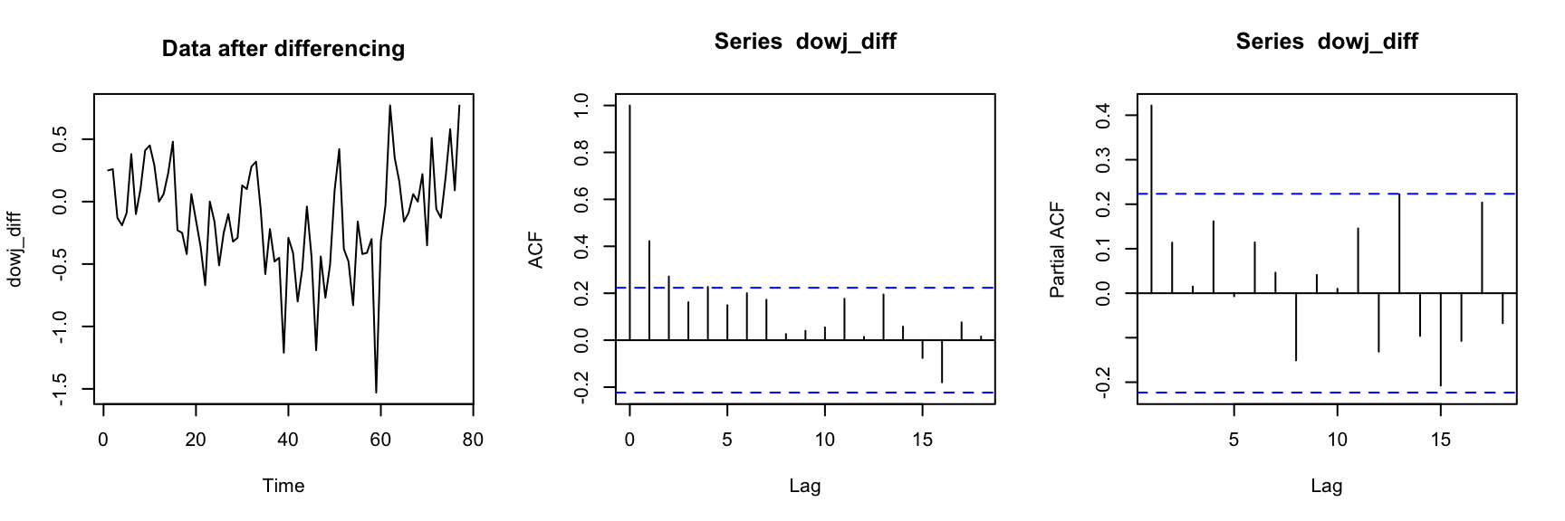

ARIMA Models

ARIMA model: definition

Autoregressive integrated moving-average models (ARIMA): Let $d \in N$ , then series ${X_{t}}$ is an ARIMA $(p, d, q)$ process if $Y_{t} = (1 - B)^{d} X_{t}$ is a causal ARMA $(p, q)$ process.
Difference equation (DE) for an ARIMA $(p, d, q)$ process $ϕ^{*} (B) X_{t} = ϕ (B) (1 - B)^{d} X_{t} = θ (B) Z_{t}, {Z_{t}} \sim WN (0, σ^{2})$
- $ϕ (z)$ : polynomial of degree $p$ , and $ϕ (z) \neq 0$ for $| z | \leq 1$
- $θ (z)$ : polynomial of degree $q$
- $ϕ^{*} (z) = ϕ (z) (1 - z)^{d}$ : has a zero of order $d$ at $z = 1$
An ARIMA process with $d > 0$ is NOT stationary!

ARIMA mean is not dertermined by the DE

${X_{t}}$ is an ARIMA $(p, d, q)$ process. We can add an arbitrary polynomial trend of degree $d - 1$ $W_{t} = X_{t} + A_{0} + A_{1} t + \dots + A_{d - 1} t^{d - 1}$ with $A_{0}, \dots, A_{d - 1}$ being any random variables, and ${W_{t}}$ still satisfies the same ARIMA $(p, d, q)$ difference equation
In other words, the ARIMA DE determines the second-order properties of ${(1 - B)^{d} X_{t}}$ but not those of ${X_{t}}$
- For parameter estimation: $ϕ$ , $θ$ , and $σ^{2}$ are estimated based on ${(1 - B)^{d} X_{t}}$ rather than ${X_{t}}$
- For forecast, we need additional assumptions

Fit data using ARIMA processes

Whether to fit a finite time series using
- non-stationary models (such as ARIMA), or
- directly using stationary models (such as ARMA)?
If the fitted stationary ARMA model’s $ϕ (\cdot)$ have zeros very close to unit circles, then fitting an ARIMA model is better
- Parameter estimation is stable
- The differenced series may only need a low-order ARMA
Limitation of ARIMA: only permits data to be nonstationary in a very special way
- Non-stationary: can have zeros anywhere on the unit circle $| z | = 1$
- ARIMA model: only has a zero of multiplicity $d$ at the point $z = 1$

Transformation and Identification Techniques

Natural log transformation

When data variance increases with mean, it’s common to apply log transformation before fitting the data using ARIMA or ARMA.
When does log transfomation work well? Suppose that $E (X_{t}) = μ_{t}, V a r (X_{t}) = σ^{2} μ_{t}^{2}$ Then by first-order Taylor expansion of $\log (X_{t})$ at $μ_{t}$ : $\log (X_{t}) \approx \log (μ_{t}) + \frac{X_{t} - μ_{t}}{μ_{t}} ⟹ V a r [\log (X_{t})] \approx \frac{V a r (X_{t})}{μ_{t}^{2}} = σ^{2}$ The data after log transformation $\log (X_{t})$ has a constant variance
Note: log transformation can only be applied to positive data
Note: If $Y_{t} = \log (X_{t})$ , then because expectation and logarithm are not interchangeable, ${\hat{X}}_{t} \neq \exp ({\hat{Y}}_{t})$

Generalize the log transformation: Box-Cox transformation

Box-Cox transformation $f_{λ} (x) = {\begin{cases} \frac{x^{λ} - 1}{λ}, & x \geq 0, λ > 0 \\ \log (x), & x > 0, λ = 0 \end{cases}$
- Usual range: $0 \leq λ \leq 1.5$
- Common values: $λ = 0, 0.5$
Note: $lim_{λ \to 0} f_{λ} (x) = \log (x)$
Box-Cox transformation can only be applied to non-negative data

Unit Root Test

Unit root test for AR $(1)$ process

${X_{t}}$ is an AR $(1)$ process: $X_{t} - μ = ϕ_{1} (X_{t - 1} - μ) + Z_{t}$
Equivalent DE: $\nabla X_{t} = X_{t} - X_{t - 1} = ϕ_{0}^{*} + ϕ_{1}^{*} X_{t - 1} + Z_{t}$
- where $ϕ_{0}^{*} = μ (1 - ϕ_{1})$ and $ϕ_{1}^{*} = ϕ_{1} - 1$
- Regressing $\nabla X_{t}$ onto $1$ and $X_{t - 1}$ , we get the OLS estimator ${\hat{ϕ}}_{1}^{*}$ and its standard error $S E ({\hat{ϕ}}_{1}^{*})$
Augmented Dickey-Fuller test for AR $(1)$
- Hypotheses: $H_{0} : ϕ_{1} = 1 ⟷ H_{1} : ϕ_{1} < 1$
- Equivalent hypotheses: $H_{0} : ϕ_{1}^{*} = 0 ⟷ H_{1} : ϕ_{1}^{*} < 0$
- Test statistic: limit distribution under $H_{0}$ is not normal or t $\hat{τ} = \frac{{\hat{ϕ}}_{1}^{*}}{S E ({\hat{ϕ}}_{1}^{*})}$
- Rejection region: reject $H_{0}$ if ${\begin{cases} \hat{τ} < - 2.57 & (90 %) \\ \hat{τ} < - 2.86 & (95 %) \\ \hat{τ} < - 3.43 & (99 %) \end{cases}$

Unit root test for AR $(p)$ process

AR $(p)$ process: $X_{t} - μ = ϕ_{1} (X_{t - 1} - μ) + \dots + ϕ_{p} (X_{t - p} - μ) + Z_{t}$
Equivalent DE: $\nabla X_{t} = ϕ_{0}^{*} + ϕ_{1}^{*} X_{t - 1} + ϕ_{2}^{*} \nabla X_{t - 1} + \dots + ϕ_{p}^{*} \nabla X_{t - p + 1} + Z_{t}$
- where $ϕ_{0}^{*} = μ (1 - \sum_{i = 1}^{p} ϕ_{i})$ , $ϕ_{1}^{*} = \sum_{i = 1}^{p} ϕ_{i} - 1$ , and $ϕ_{j}^{*} = - \sum_{i = j}^{p} ϕ_{i}$ for $j \geq 2$
- Regressing $\nabla X_{t}$ onto $1, X_{t - 1}, \nabla X_{t - 1}, \dots, \nabla X_{t - p + 1}$ , we get the OLS estimator ${\hat{ϕ}}_{1}^{*}$ and its standard error $S E ({\hat{ϕ}}_{1}^{*})$
Augmented Dickey-Fuller test for AR $(p)$
- Hypotheses: $H_{0} : ϕ_{1}^{*} = 0 ⟷ H_{1} : ϕ_{1}^{*} < 0$
- Test statistic: $\hat{τ} = \frac{{\hat{ϕ}}_{1}^{*}}{S E ({\hat{ϕ}}_{1}^{*})}$
- Rejection region: same as augmented Dickey-Fuller test for AR $(1)$

Implement augmented Dickey-Fuller test in R

library(tseries);
## Note: the lag k here is the AR order p
adf.test(dowj, k = 2);

## 
##  Augmented Dickey-Fuller Test
## 
## data:  dowj
## Dickey-Fuller = -1.3788, Lag order = 2, p-value = 0.8295
## alternative hypothesis: stationary

Forecast ARIMA models

Forecast an ARIMA $(p, 1, q)$ process

${X_{t}}$ is ARIMA $(p, 1, q)$ , and ${Y_{t} = \nabla X_{t}}$ is a causal ARMA $(p, q)$ $X_{t} = X_{0} + \sum_{j = 1}^{t} Y_{j}, t = 1, 2, \dots$
Best linear predictor of $X_{n + 1}$ $P_{n} X_{n + 1} = P_{n} (X_{0} + Y_{1} + \dots + Y_{n + 1}) = P_{n} (X_{n} + Y_{n + 1}) = X_{n} + P_{n} (Y_{n + 1}),$
- $P_{n}$ means based on ${1, X_{0}, X_{1}, \dots, X_{n}}$ , or equivalently, ${1, X_{0}, Y_{1}, \dots, Y_{n}}$
- To find $P_{n} (Y_{n + 1})$ , we need to know $E (X_{0}^{2})$ and $E (X_{0} Y_{j})$ , for $j = 1, \dots, n + 1$ .
A sufficient assumption for $P_{n} (Y_{n + 1})$ to be the best linear predictor in term of ${Y_{1}, \dots, Y_{n}}$ : $X_{0}$ is uncorrelated with $Y_{1}, Y_{2}, \dots$

Forecast an ARIMA $(p, d, q)$ process

The observed ARIMA $(p, d, q)$ process ${X_{t}}$ satisfies $Y_{t} = (1 - B)^{d} X_{t}, t = 1, 2, \dots, {Y_{t}} \sim causal ARMA (p, q)$
Assumption: the random vector $(X_{1 - d}, \dots, X_{0})$ is uncorrelated with $Y_{t}$ for all $t > 0$
One-step predictors ${\hat{Y}}_{n + 1} = P_{n} Y_{n + 1}$ and ${\hat{X}}_{n + 1} = P_{n} X_{n + 1}$ : $X_{n + 1} - {\hat{X}}_{n + 1} = Y_{n + 1} - {\hat{Y}}_{n + 1}$
Recall: the $h$ -step predictor of ARMA $(p, q)$ for $n > max (p, q)$ : $P_{n} Y_{n + h} = \sum_{i = 1}^{p} ϕ_{i} P_{n} Y_{n + h - i} + \sum_{j = h}^{q} θ_{n + h - 1, j} (Y_{n + h - j} - {\hat{Y}}_{n + h - j})$
$h$ -step predictor of ARIMA $(p, d, q)$ for $n > max (p, q)$ : $P_{n} X_{n + h} = \sum_{i = 1}^{p + d} ϕ_{i}^{*} P_{n} X_{n + h - i} + \sum_{j = h}^{q} θ_{n + h - 1, j} (X_{n + h - j} - {\hat{X}}_{n + h - j})$ where $ϕ^{*} (z) = (1 - z)^{d} ϕ (z) = 1 - ϕ_{1}^{*} z - \dots - ϕ_{p + d}^{*} z^{p + d}$

Seasonal ARIMA Models

Seasonal ARIMA (SARIMA) Model: definition

Suppose $d, D$ are non-negative integers. ${X_{t}}$ is a seasonal ARIMA $(p, d, q)$ $\times$ $(P, D, Q)_{s}$ process with period $s$ if the differenced series $Y_{t} = (1 - B)^{d} (1 - B^{s})^{D} X_{t}$ is a causal ARMA process defined by $ϕ (B) Φ (B^{s}) Y_{t} = θ (B) Θ (B^{s}) Z_{t}, {Z_{t}} \sim WN (0, σ^{2})$ where $\begin{aligned} ϕ (z) & = 1 - ϕ_{1} z - \dots - ϕ_{p} z^{p}, Φ (z) = 1 - Φ_{1} z - \dots - Φ_{P} z^{P} \\ θ (z) & = 1 + θ z + \dots + θ_{q} z^{q}, Θ (z) = 1 + Θ z + \dots + Θ_{Q} z^{Q} \end{aligned}$
${Y_{t}}$ is causal if and only if neither $ϕ (z)$ or $Φ (z)$ has zeros inside the unit circle
Usually, $s = 12$ for monthly data

Special case: seasonal ARMA (SARMA)

Between-year model: for monthly data, each one of the 12 time series is generated by the same ARMA $(P, Q)$ model $Φ (B^{12}) Y_{t} = Θ (B^{12}) U_{t}, {U_{j + 12 t}, t \in Z} \sim WN (0, σ_{U}^{2})$
SARMA $(P, Q)$ with period $s$ : in the above between-year model, the period 12 can be changed to any positive integer $s$
- If ${U_{t}, t \in Z} \sim WN (0, σ_{U}^{2})$ , then the ACVF $γ (h) = 0$ unless $h$ divides $s$ evenly. But this may not be ideal for real life application! E.g., this Feb is correlated with last Feb, but not this Jan.
General SARMA $(p, q)$ $\times$ $(P, Q)$ with period $s$ : incorporate dependency between the 12 series by letting ${U_{t}}$ be ARMA: $Φ (B^{s}) Y_{t} = Θ (B^{s}) U_{t}, ϕ (B) U_{t} = θ (B) Z_{t}, {Z_{t}} \sim WN (0, σ^{2})$
- Equivalent DE for the general SARMA: $ϕ (B) Φ (B^{s}) Y_{t} = θ (B) Θ (B^{s}) Z_{t}$

Fit a SARIMA Model

Period $s$ is known

Find $d$ and $D$ to make the difference series ${Y_{t}}$ to look stationary
Examine the sample ACF and sample PACF of ${Y_{t}}$ at lags being multiples of $s$ , to find orders $P, Q$
Use $\hat{ρ} (1), \dots, \hat{ρ} (s - 1)$ to find orders $p, q$
Use AICC to decide among competing order choices
Given orders $(p, d, q, P, D, Q)$ , estimate MLE of parameters $(ϕ, θ, Φ, Θ, σ^{2})$

Regression with ARMA Errors

Regression with ARMA errors: OLS estimation

Linear model with ARMA errors $W = (W_{1}, \dots, W_{n})^{'}$ : $Y_{t} = x_{t}^{'} β + W_{t}, t = 1, \dots, n, {W_{t}} \sim causal ARMA (p, q)$
- Note: each row is indexed by a different time $t$ !
- Error covariance $Γ_{n} = E (W W^{'})$
Ordinary least squares (OLS) estimator ${\hat{β}}_{OLS} = (X^{'} X)^{- 1} X^{'} Y$
- Estimated by minimizing $(Y - X β)^{'} (Y - X β)$
- OLS is unbiased, even when errors are dependent!

Regression with ARMA errors: GLS estimation

Generalized least squares (GLS) estimator ${\hat{β}}_{GLS} = (X^{'} Γ_{n}^{- 1} X)^{- 1} X^{'} Γ_{n}^{- 1} Y$
- Estimated by minimizing the weighted sum of squares $(Y - X β)^{'} Γ_{n}^{- 1} (Y - X β)$
- Covariance $Cov ({\hat{β}}_{GLS}) = (X^{'} Γ_{n}^{- 1} X)^{- 1}$
- GLS is the best linear unbiased estimator, i.e., for any vector $c$ and any unbiased estimator $\hat{β}$ , we have $Var (c^{'} {\hat{β}}_{GLS}) \leq Var (c^{'} \hat{β})$

When ${W_{t}}$ is an AR $(p)$ process

We can apply $ϕ (B)$ to each side of the regression equation and get uncorrelated, zero-mean, constant-variance errors $ϕ (B) Y = ϕ (B) X β + ϕ (B) W = ϕ (B) X β + Z$
Under the transformed target variable $Y_{t}^{*} = ϕ (B) Y_{t}, t = p + 1, \dots, n$ and the transformed design matrix $X_{t, j}^{*} = ϕ (B) X_{t, j}, t = p + 1, \dots, n, j = 1, \dots, k$ the OLS estimator is the best linear unbiased estimator
Note: after the transformation, the regression sample size reduces to $n - p$

Regression with ARMA errors: MLE

MLE of $β, ϕ, θ, σ^{2}$ can be estimated by maximizing the Gaussian likelihood with error covariance $Γ_{n}$
An iterative scheme
1. Compute ${\hat{β}}_{OLS}$ and regression residuals $Y - X {\hat{β}}_{OLS}$
2. Based on the estimated residuals, compute MLE of the ARMA $(p, q)$ parameters
3. Based on the fitted ARMA model, compute ${\hat{β}}_{GLS}$
4. Compute regression residuals $Y - X {\hat{β}}_{GLS}$ , and return to Step 2 until estimators stabilize
Asymptotic properties of MLE: If ${W_{t}}$ is a causal and invertible ARMA, then
- MLEs are asymptotically normal
- Estimated regression coefficients are asymptotically independent of estimated ARMA parameters

References

Brockwell, Peter J. and Davis, Richard A. (2016), Introduction to Time Series and Forecasting, Third Edition. New York: Springer
Weigt, George (2018) ITSM-R Reference Manual http://www.eigenmath.org/itsmr-refman.pdf
R package tseries https://cran.r-project.org/web/packages/tseries/index.html

Book Notes: Intro to Time Series and Forecasting -- Ch6 ARIMA Models

When data is not stationary

A non-stationary exmaple: Dow Jones utilities index data

After differencing

ARIMA Models

ARIMA model: definition

ARIMA mean is not dertermined by the DE

Fit data using ARIMA processes

Transformation and Identification Techniques

Natural log transformation

Generalize the log transformation: Box-Cox transformation

Unit Root Test

Unit root test for AR(1)(1) process

Unit root test for AR(p)(p) process

Implement augmented Dickey-Fuller test in R

Forecast ARIMA models

Forecast an ARIMA(p,1,q)(p,1,q) process

Forecast an ARIMA(p,d,q)(p,d,q) process

Seasonal ARIMA Models

Seasonal ARIMA (SARIMA) Model: definition

Special case: seasonal ARMA (SARMA)

Fit a SARIMA Model

Regression with ARMA Errors

Regression with ARMA errors: OLS estimation

Regression with ARMA errors: GLS estimation

When {Wt}{Wt} is an AR(p)(p) process

Regression with ARMA errors: MLE

References

Unit root test for AR $(1)$ process

Unit root test for AR $(p)$ process

Forecast an ARIMA $(p, 1, q)$ process

Forecast an ARIMA $(p, d, q)$ process

When ${W_{t}}$ is an AR $(p)$ process