K-means clustering: problem

• Data

  • $D$-dimensional observations: $x_1,\dots ,x_N$

• Parameters

  • $K$ clusters’ means: ${\mu }_1,\dots ,{\mu }_K$
  • Binary indicator $r_{nk}\in \{0,1\}$: if object $n$ is in class $k$

• Goal: find values for $\left\{{\mu }_k\right\}$ and $\left\{r_{nk}\right\}$ to minimize the objective function (called a distortion measure) $$J=\sum _{n=1}^N\sum _{k=1}^K{r}_{nk}\parallel x_n-{\mu }_k{\parallel }^2$$

K-means clustering: solution

• Two-stage optimization

  • Update $r_{nk}$ and ${\mu }_k$ alternatively, and repeat until convergence
  • Resembles the E step and M step in the EM algorithm

1. E(expectation) step: updates $r_{nk}$.

   • Assign the $n$th data point to the closest cluster center $$r_{nk}=\{\begin{array}{cc}1& \text{if}k=\arg {min}_j\parallel x_n-{\mu }_k{\parallel }^2\\ 0& \text{otherwise}\end{array}$$

2. M(maximization) step: updates ${\mu }_k$

   • Set cluster mean to be mean of all data points assigned to this cluster $${\mu }_k=\frac{{\sum }_n{r}_{nk}{x}_n}{{\sum }_n{r}_{nk}}$$

Mixture of Gaussians: definition

• Mixture of Gaussians: log likelihood $$\log p\left(x\right)=\log \{\sum _{k=1}^K{\pi }_k\cdot \text{N}(x\mid {\mu }_k,{\Sigma }_k)\}$$

• Introduce a $K$-dim latent indicator variable $z\in \{0,1{\}}^K$ $$z_k=1\left(\text{if}x\text{is from the}k\text{-th Gaussian component}\right)$$

The marginal distribution of $z$ is multinomial $$p(z_k=1)={\pi }_k$$

• We call the posterior probability as the Responsibility that component $k$ takes for explaining the observation $x$ $$\gamma \left(z_k\right)=p(z_k=1\mid x)=\frac{{\pi }_k\cdot \text{N}(x\mid {\mu }_k,{\Sigma }_k)}{{\sum }_{j=1}^K{\pi }_j\cdot \text{N}(x\mid {\mu }_j,{\Sigma }_j)}$$

Mixture of Gaussians: singularity problem with MLE

• Problem with maximum likelihood estimation: presence of singularities: there will be clusters that contains only one data point, so that the corresponding covariance matrix will be estimated at zero, thus the likelihood explodes

  • Therefore, when finding MLE, we should avoid finding such singularity solution and instead seek well-behaved local maxima of the likelihood function: see the following EM approach

  • Alternatively, we can to adopt a Bayesian approach

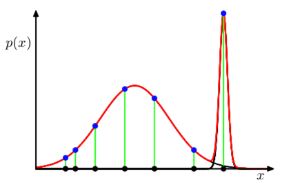
Figure 1: Illustration of singularities

Conditional MLE of ${\mu }_k$

• Suppose we observe $N$ data points $X=\{x_1,\dots ,x_N\}$

• Similarly, we write the $N$ latent variables as $Z=\{z_1,\dots ,z_N\}$

• Set the derivatives of $\log p(X\mid \pi ,\mu ,\Sigma )$ with respect to $\mu$ to zero $$0=\sum _{n=1}^N\gamma \left(z_{nk}\right){\Sigma }_k(x_n-{\mu }_k)$$ Then we obtain $${\mu }_k=\frac{1}{N_k}\sum _{n=1}^N\gamma \left(z_{nk}\right)x_n$$ where $N_k$ is the effective number of points assigned to cluster $k$ $$N_k=\sum _{n=1}^N\gamma \left(z_{nk}\right)$$

Conditional MLE of ${\Sigma }_k$ and ${\pi }_k$

• Similarly, setting the derivatives of log likelihood wrt ${\Sigma }_k$, we have $${\Sigma }_k=\frac{1}{N_k}\sum _{n=1}^N\gamma \left(z_{nk}\right)(x_n-{\mu }_k){(x_n-{\mu }_k)}^{\top }$$

• Use Lagrange multiplier to maximize log likelihood wrt ${\pi }_k$ under the constraint that all ${\pi }_k$ add up to one: $$\log p(X\mid \pi ,\mu ,\Sigma )+\lambda (\sum _{k=1}^K{\pi }_k-1)$$ we get the solution $${\pi }_k=\frac{N_k}{N}$$

• The above results on ${\mu }_k,{\Sigma }_k,{\pi }_k$ are not closed-form solution because the responsibilities $\gamma \left(z_{nk}\right)$ depend on them in a complex way.

EM algorithm for mixture of Gaussians

1. Initialize ${\mu }_k,{\Sigma }_k,{\pi }_k$, usually using the $K$-means algorithm.

2. E step: compute responsibilities using the current parameters $$\gamma \left(z_{nk}\right)=\frac{{\pi }_k\cdot \text{N}(x_n\mid {\mu }_k,{\Sigma }_k)}{{\sum }_{j=1}^K{\pi }_j\cdot \text{N}(x_n\mid {\mu }_j,{\Sigma }_j)}$$

3. M step: re-estimate the parameters using the current responsibilities, where $N_k={\sum }_{n=1}^N\gamma \left(z_{nk}\right)$ $$\begin{array}{cc}{\mu }_k^{\text{new}}& =\frac{1}{N_k}\sum _{n=1}^N\gamma \left(z_{nk}\right)x_n\\ {\Sigma }_k^{\text{new}}& =\frac{1}{N_k}\sum _{n=1}^N\gamma \left(z_{nk}\right)(x_n-{\mu }_k){(x_n-{\mu }_k)}^{\top }\\ {\pi }_k^{\text{new}}& =\frac{N_k}{N}\end{array}$$

4. Check for convergence of either the parameters or the log likelihood. If not converged, return to step 2.

Connection between K-means and Gaussian mixture model

• K-means algorithm itself is often used to initialize the parameters in a Gaussian mixture model before applying the EM algorithm

• Mixture of Gaussians: soft assignment of data points to clusters, using posterior probabilities

• $K$-means can be viewed as a special case of mixture of Gaussian, where covariances of mixture components are $ϵI$, where $ϵ$ is a parameter shared by all components.

  • In the responsibility calculation, $$\gamma \left(z_{nk}\right)=\frac{{\pi }_k\exp \{-\parallel x_n-{\mu }_k{\parallel }^2/2ϵ\}}{{\sum }_j{\pi }_j\exp \{-\parallel x_n-{\mu }_j{\parallel }^2/2ϵ\}}$$ In the limit $ϵ\to 0$, for each observation $n$, the responsibilities $\left\{\gamma \right(z_{nk}),k=1,\dots ,K\}$ has exactly one unity and all the rest are zero.

EM algorithm: definition

• Goal: maximize likelihood $p(X\mid \theta )$ with respect to the parameter $\theta$, for models having latent variables $Z$.

• Notations
  • $X$: observed data; also called incomplete data
  • $\theta$: model parameters
  • $Z$: latent variables, usually each observation has a latent variable
  • $\{X,Z\}$ is called complete data
• Log likelihood $$\log p(X\mid \theta )=\log \left\{\sum _{Z}p\right(X,Z\mid \theta \left)\right\}$$
  • The sum over $Z$ can be replaced by an integral if $Z$ is continuous
  • The presence of sum prevents the logarithm from acting directly on the joint distribution. This complicates MLE solutions, especially for exponential family.

General EM algorithm: two-stage iterative optimization

1. Choose the initial parameters ${\theta }^{\text{old}}$

2. E step: since the conditional posterior $p(Z\mid X,{\theta }^{\text{old}})$ contains all of our knowledge about the latent variable $Z$, we compute the expected complete-data log likelihood under it. $$\begin{array}{cc}Q(\theta ,{\theta }^{\text{old}})& =E_{Z\mid X,{\theta }^{\text{old}}}\left\{\log p\right(X,Z\mid \theta \left)\right\}\\ & =\sum _{Z}p(Z\mid X,{\theta }^{\text{old}})\log p(X,Z\mid \theta )\end{array}$$

3. M step: revise parameter estimate $${\theta }^{\text{new}}=\arg \underset{\theta }{max}Q(\theta ,{\theta }^{\text{old}})$$
   • Note in the maximizing step, the logarithm acts driectly on the joint likelihood $p(X,Z\mid \theta )$, so the maximizating will be tractable.

4. Check for convergence of the log likelihood or the parameter values. If not converged, use ${\theta }^{\text{new}}$ to replace ${\theta }^{\text{old}}$, and return to step 2.

Gaussian mixtures revisited

• Recall that latent variables $Z\in R^{N\times K}$ : $$z_{nk}=1\left(\text{if}{x}_n\text{is from the}k\text{-th Gaussian component}\right)$$
• Complete data log likelihood $$\log p(X,Z\mid \mu ,\Sigma ,\pi )=\sum _{n=1}^N\sum _{k=1}^K{z}_{nk}\{\log {\pi }_k+\log \text{N}(x_n\mid {\mu }_k,{\Sigma }_k)\}$$
  • Comparing this with incomplete data log likelihood in Eq , we have the sum over $k$ and logarithm interchanged. Thus, the logarithm acts on Gaussian density directly.

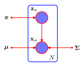
Figure 2: Mixture of Gaussians, treating latent variables as observed

Continue: Gaussian mixtures revisited

• Conditional posterior of $Z$ $$p(Z\mid X,\mu ,\Sigma ,\pi )\propto \prod _{n=1}^N\prod _{k=1}^K{\left[{\pi }_k\text{N}(x_n\mid {\mu }_k,{\Sigma }_k)\right]}^{z_{nk}}$$ Thus, the conditional posterior of $\left\{z_n\right\}$ are independent

• Conditional expectations $$E_{Z\mid X,{\mu }^{\text{old}},{\Sigma }^{\text{old}},{\pi }^{\text{old}}}{z}_{nk}=\gamma (z_{nk}{)}^{\text{old}}$$

• Thus the objective function in the M-step $$\begin{array}{cc}& E_{Z\mid X,{\mu }^{\text{old}},{\Sigma }^{\text{old}},{\pi }^{\text{old}}}\log p(X,Z\mid \mu ,\Sigma ,\pi )\\ =& \sum _{n=1}^N\sum _{k=1}^K\gamma (z_{nk}{)}^{\text{old}}\{\log {\pi }_k+\log \text{N}(x_n\mid {\mu }_k,{\Sigma }_k)\}\end{array}$$

A different view of the EM algorithm

• Goal: maximize the incomplete data likelihood $$p(X\mid \theta )=\sum _{Z}p(X,Z\mid \theta )$$

• Suppose that optimization of $p(X\mid \theta )$ is difficult, but optimization of $p(X,Z\mid \theta )$ is significantly easier.

• An important decompsition: holds for any arbitrary distribution $q\left(Z\right)$ $$\log p(X\mid \theta )=L(q,\theta )+\text{KL}(q\parallel p)$$ where $L(q,\theta )$ is called a lower bound on $\log p(X\mid \theta )$: $$\begin{array}{cc}L(q,\theta )& =\sum _{Z}q\left(Z\right)\log \left\{\frac{p(X,Z\mid \theta )}{q\left(Z\right)}\right\}\\ \text{KL}(q\parallel p)& =-\sum _{Z}q\left(Z\right)\log \left\{\frac{p(Z\mid X,\theta )}{q\left(Z\right)}\right\}\end{array}$$

  • Note: this formula will appear again in variational inference.

A different view of the EM algorithm: E step

• In E step, the lower bound $L(q,{\theta }^{\text{old}})$ is maximized with respect to $q\left(Z\right)$ while keeping ${\theta }^{\text{old}}$ fixed

• The solution is when the KL divergence $\text{KL}\left(q\right(Z)\parallel p(Z\mid X,{\theta }^{\text{old}}))$ is zero, i.e., $$q\left(Z\right)=p(Z\mid X,{\theta }^{\text{old}})$$

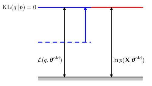
Figure 3: In the E step, the lower bound moves to the same value as the old incomplete data log likelihood

A different view of the EM algorithm: M step

• In M step, the distribution $q\left(Z\right)$ is held fixed and the lower bound $L(q,{\theta }^{\text{old}})$ is maximized wrt $\theta$ to give some new value ${\theta }^{\text{new}}$. Thus, the lower bound increases.

• Since $q\left(Z\right)$ is fixed at ${\theta }^{\text{old}}$, it will not equal the new posterior $p(Z\mid X,{\theta }^{\text{new}})$. Therefore, the KL divergence becomes nonzero.

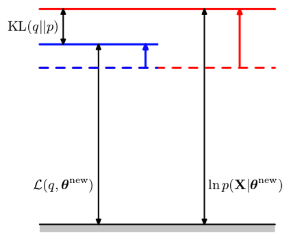
Figure 4: In the M step, both the lower bound and the KL divergence increase.

EM algorithm illustration

• Red curve: incomplete data log likelihood
• Blue curve: lower bound $L(\theta ,{\theta }^{\text{old}})$
• Green curve: lower bound $L(\theta ,{\theta }^{\text{new}})$
• The lower bounds have tangential contacts with the log likelihood

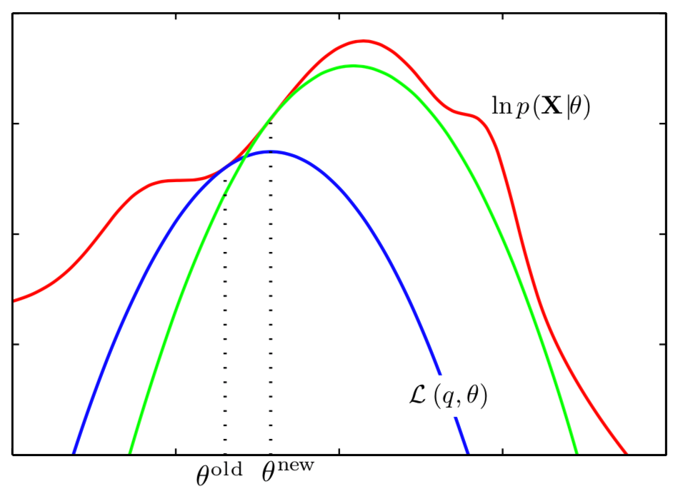
Figure 5: Illustration of EM algorithm, in the parameter space

EM algorithm in Bayesian statistics

• EM algorithm can be used to estimate maximum posterior (MAP)

• In this case, the objective function is $$p(\theta \mid X)\propto p(X\mid \theta )p\left(\theta \right)$$ Hence, the expectation in Step 2 becomes $$\begin{array}{cc}Q(\theta ,{\theta }^{\text{old}})& =E_{Z\mid X,{\theta }^{\text{old}}}\left\{\log p\right(X,Z\mid \theta )+\log p(\theta \left)\right\}\\ & =E_{Z\mid X,{\theta }^{\text{old}}}\left\{\log p\right(X,Z\mid \theta \left)\right\}+\log p\left(\theta \right)\end{array}$$

EM algorithm and missing data

• The latent variables can be the missing values in the data
• This is valid is the data are missing at random

EM algorithm for IID data with $N$ latent variables

• Suppose $N$ data points $\{x_1,\dots ,x_N\}$ are IID

• Each observation $x_n$ has its corresponding latent variable $z_n$

• Then the conditional posterior of $Z$ also factorizes wrt $n$: $$p(Z\mid X,\theta )=\prod _{n=1}^{N}p(z_n\mid x_n,\theta )$$

• Exploit this structure: using incremental form of EM that at each cycle only process one data point
  • Benefit: no need to wait for the whole data set to finish processing

Extensions of EM algorithms

• For complex models, E step and/or M step can be intractable

• Generalized EM (GEM): address an intractable M step
  • Instead of maximizing the objective function in the M step, just changing the parameter to increase its value
  • E.g., using nonlinear optimization methods such as conjugate gradients algorithm
  • E.g., expected conditional maximization (ECM), constrained optimization

• We can also generalize the E step: find $q\left(Z\right)$ to partially, rather than completely, optimize $L(q,\theta )$

References

• Bishop, C. M. (2006). Pattern Recognition and Machine Learning. Springer.