Four methods to impute under the normal linear model

1. Regression imputation: Predict (bad!). Fit a linear model on the observed data and get the OLS estimates ${\hat{\beta }}_0,{\hat{\beta }}_1$. Impute with the predicted values $$\dot{y}={\hat{\beta }}_0+X_{\text{mis}}{\hat{\beta }}_1$$
   • In mice package, this method is norm.predict
2. Stochastic regression imputation: Predict + noise (better, but still bad). Also add a random drawn noise from the estimated residual normal distribution $$\dot{y}={\hat{\beta }}_0+X_{\text{mis}}{\hat{\beta }}_1+\dot{ϵ},\dot{ϵ}\sim \text{N}(0,{\hat{\sigma }}^2)$$
   • In mice package, this method is norm.nob

Method 3: Bayesian multiple imputation

• Predict + noise + parameter uncertainty $$\dot{y}={\dot{\beta }}_0+X_{\text{mis}}{\dot{\beta }}_1+\dot{ϵ},\dot{ϵ}\sim \text{N}(0,{\dot{\sigma }}^2)$$

• Under the priors (where the hyper-parameter $\kappa$ is fixed at a small value, e.g., $\kappa =0.0001$) $$\beta \sim \text{N}(0,I_p/\kappa ),p\left({\sigma }^2\right)\propto 1/{\sigma }^2$$ We draw $\dot{\beta }$ (including both ${\dot{\beta }}_0$ and ${\dot{\beta }}_1$), $\dot{{\sigma }^2}$ from the posterior distribution

• In mice package, this method is norm

Method 4: Bootstrap multiple imputation

• Predict + noise + parameter uncertainty $$\dot{y}={\dot{\beta }}_0+X_{\text{mis}}{\dot{\beta }}_1+\dot{ϵ},\dot{ϵ}\sim \text{N}(0,{\dot{\sigma }}^2)$$ where ${\dot{\beta }}_0$, ${\dot{\beta }}_1$, and $\dot{{\sigma }^2}$ are OLS estimates calculated form a bootstrap sample taken from the observed data

• In mice package, this method is norm.boot

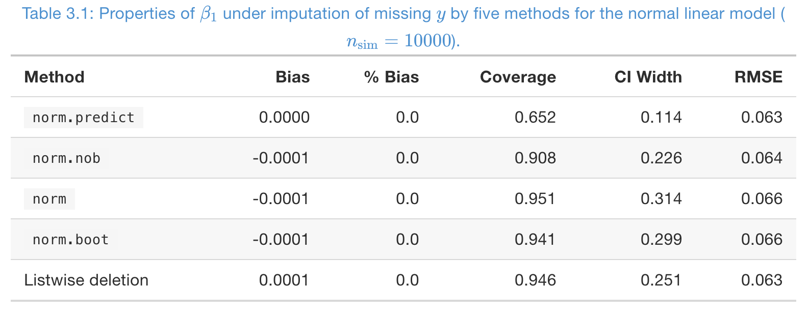
A simulation study, to impute MCAR missing in $y$

• Missing rate $50\%$ in $y$, and number of imputations $m=5$.
  • From coverage, norm, norm.boot, and listwise deletion are good
  • From CI width, listwise deletion is better than multiple imputation here, but it’s not always this case, especially when the number of covariates is large.
  • RMSE is not imformative at all!

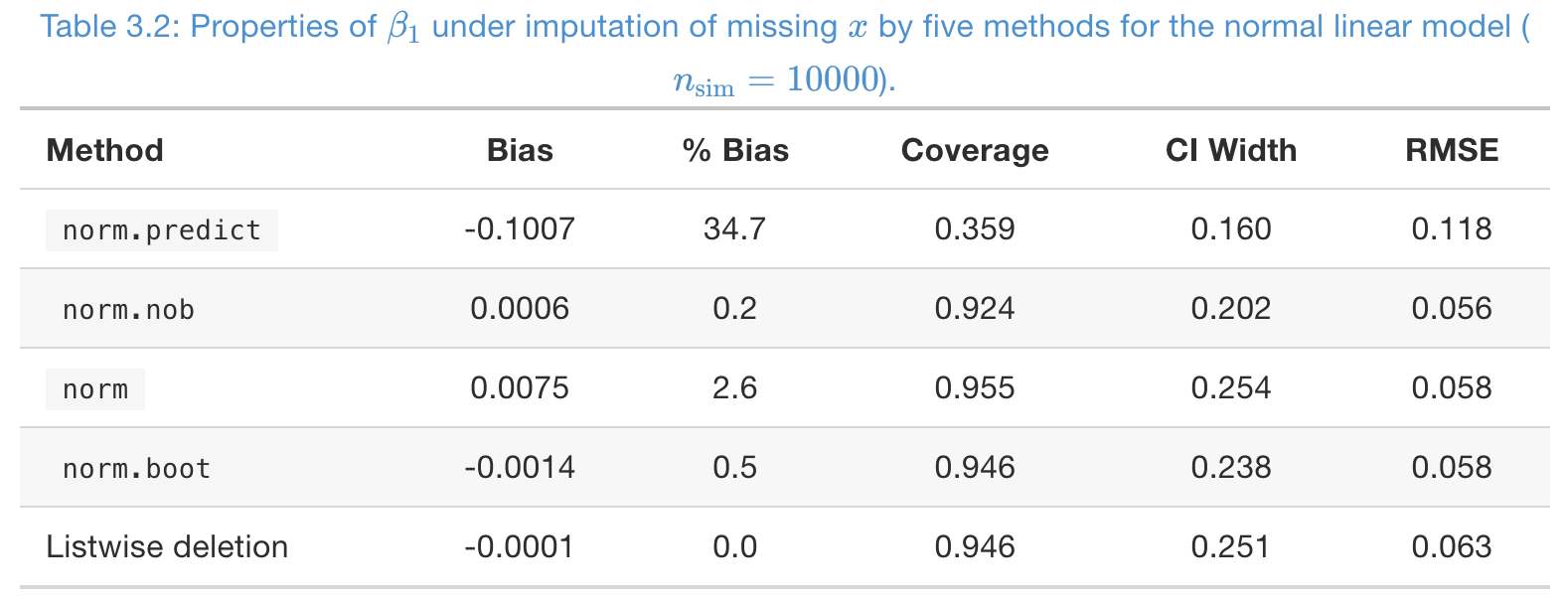
### A simulation study, to impute MCAR missing in $x$

• Missing rate $50\%$ in $x$, and number of imputations $m=5$.
  • norm.predict is severely biased; norm is slightly biased
  • From coverage, norm, norm.boot, and listwise deletion are good
  • Again, RMSE is not imformative at all!

Impute from a (continuous) non-normal distributions

• Optional 1: mean predictive matching

• Optional 2: model the non-normal data directly
  • E.g., impute from a t-distribution
  • The GAMLSS package: extends GLM and GAM

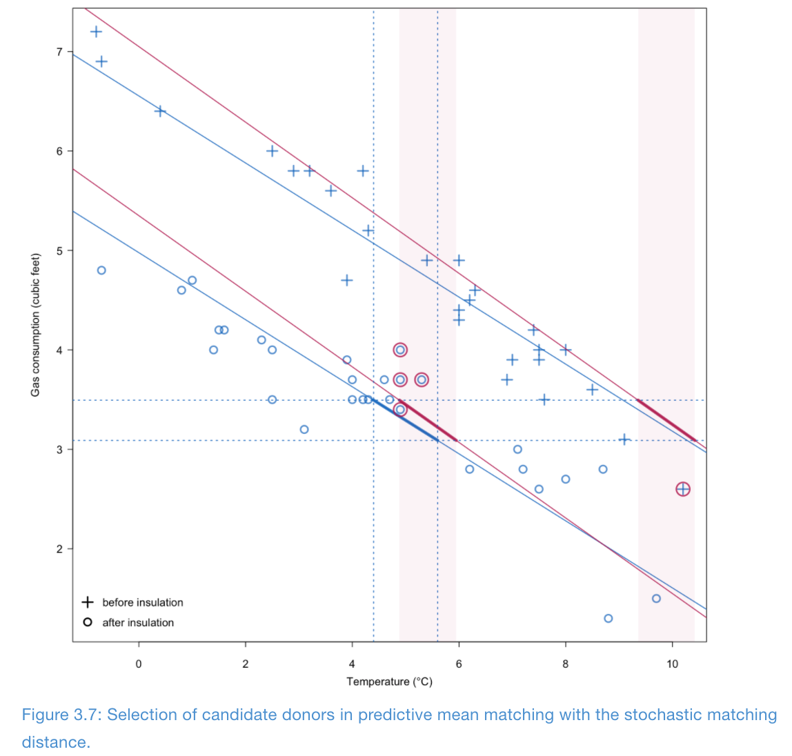
Predictive mean matching (PMM), general principle

• For each missing entry, the method forms a small set of candidate donors (3, 5, or 10) from completed cases whose predicted values closest to the predicted value for the missing entry

• One donor is randomly drawn from the candidates, and the observed value of the donor is taken to replace the missing value

Advantages of predictive mean matching (PMM)

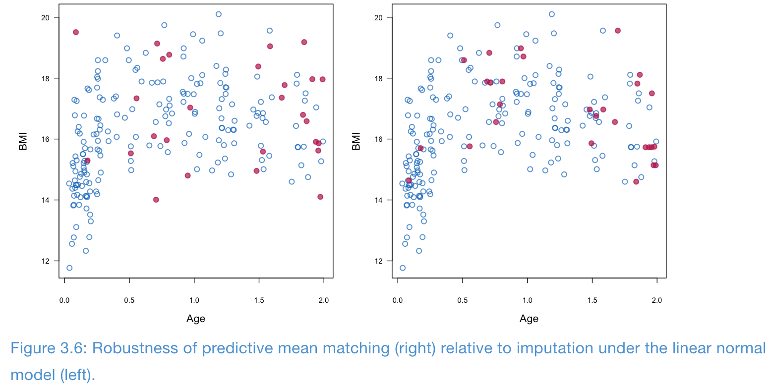
• PMM is fairly robust to transformations of the target variable

• PMM can also be used for discrete target variables

• PMM is fairly robust to model misspecification
  • In the following example, the relationship between age and BMI is not linear, but PMM seems to preserve this relationship better than linear normal model

How to select the donors

• Once the metric has been defined, there are four ways to select the donors.
  • Let ${\hat{y}}_i$ denote the predicted values of rows with observed $y_i$
  • Let ${\hat{y}}_j$ denote the predicted values of rows with missing $y_j$

1. Pre-specify a threshold $\eta$, take all $i$ such that $|{\hat{y}}_i-{\hat{y}}_j|<\eta$ as donors, and randomly sample one donor to impute
2. Choose the closest candidate as the donor (only 1 donor), also called (nearest neighbor hot deck)
3. Pre-specify a number $d$, take the $d$ closest candidate as donors, and randomly sample one donor to impute. Usually, $d=3,5,10$
4. Sample one donor with a probability that depends on the distance $|{\hat{y}}_i-{\hat{y}}_j|$
   • Implemented by the midastouch method in mice, and also the midastouch package

Types of matching

• Type 0: $\hat{y}=X_{\text{obs}}\hat{\beta }$ is matched to ${\hat{y}}_j=X_{\text{mis}}\hat{\beta }$
  • Bad: it ignores the sampling variability in $\hat{\beta }$
• Type 1: $\hat{y}=X_{\text{obs}}\hat{\beta }$ is matched to ${\dot{y}}_j=X_{\text{mis}}\dot{\beta }$
  • Here, $\dot{\beta }$ is a random draw from the posterior distribution
  • Good. The default in mice
• Type 2: $\dot{y}=X_{\text{obs}}\dot{\beta }$ is matched to ${\dot{y}}_j=X_{\text{mis}}\dot{\beta }$
  • Not very ideal, when model is small, the same donors get selected too often
• Type 3: $\dot{y}=X_{\text{obs}}\dot{\beta }$ is matched to ${\ddot{y}}_j=X_{\text{mis}}\ddot{\beta }$
  • Here, $\dot{\beta }$ and $\ddot{\beta }$ are two different random draws from the posterior distribution
  • Good

Illustration of Type 1 matching

Number of donors $d$

• $d=1$ is too low (bad!). It may select the same donor over and over again

• The default in mice is $d=5$. Also, $d=3,10$ are also feasible

Pitfalls of PMM

• If the data is small, or if there is a region where the missing rate is high, then the same donors may be used for too many times.

• Mis-specification of the impute model

• PMM cannot be used to extrapolate beyond the range of the data, or to interpolate within the region where data is sparse

• PMM may not perform well with small datasets

Multiple imputation under a tree model

• missForest: single imputation with CART is bad

• Multiple imputation under a tree model using the bootstrap:

1. Draw a bootstrap sample among the observed data, and fit a CART model $f\left(X\right)$
2. For each missing value $y_j$, find it’s terminal node $g_j$. All the $d_j$ cases in this node are the donors

3. Randomly select one donor to impute

   • When fitting the tree, it may be useful to pre-set the size of nodes to be 5 or 10
   • We can also use random forest instead of CART

Imputation under Bayesian GLMs

• Binary data: logistic regression (logreg method in mice)
  • In case of data separation, use a more informative Bayesian prior

• Categorical variable with $K$ unordered categories: multinomial logit model (polyreg method in mice package) $$P(y_i=k\mid X_i,\beta )=\frac{\exp \left(X_i{\beta }_k\right)}{{\sum }_{j=1}^K\exp \left(X_i{\beta }_j\right)}$$

• Categorical variable with $K$ ordered categories: ordered logit model (polr method in mice package) $$P(y_i\le k\mid X_i,\beta ,{\tau }_k)=\frac{\exp ({\tau }_k-X_i\beta )}{1+\exp ({\tau }_k-X_i\beta )}$$
  • For identifiability, set ${\tau }_1=0$

• When impute from these GLM models, make sure to not use the MLE of parameters, but either a draw from posterior, or a bootstraped estimate.

Categorical variables are harder to impute than continuous ones

• Empirically, the GLM imputations do not perform well
  • If missing rate exceeds 0.4
  • If the data is imbalanced
  • If there are many categories
• GLM imputation is found inferior than CART or latent class models

Imputation of count data

• Option 1: predictive mean matching
• Option 2: ordered categorical imputation
• Option 3: (zero-inflated) Poisson regression
• Option 4: (zero-inflated) negative binomial regression

Imputation of semi-continuous data

• Semi-continuous data: has a high mass at one point (often zero) and a continuous distribution over the remaining values

• Option 1: model the data in two parts: logistic regression + regression

• Option 2: predictive mean matching

References

• Van Buuren, S. (2018). Flexible Imputation of Missing Data, 2nd Edition. CRC press.

  • https://stefvanbuuren.name/fimd/