Sample indicator: $I=(I_1,\dots ,I_N{)}^{\prime }$; for unit $i$, $$I_i=1_{\left\{\text{unit}i\text{included in the sample}\right\}}$$

Sample selection processes can be characterized by a distribution for $I$ given $Y$ and $Z$.

Properties of probability sampling

1. Unconfounded: selection doesn’t depend on $Y$, i.e., $$f(I\mid Y,Z)=f(I\mid Z)$$

2. Every unit has a positive (known) probability of selection $${\pi }_i=P(I_i=1\mid Z)>0,\text{for all}i$$

In equal probability sample design, ${\pi }_i$ is the same for all $i$

$Z$ is a variable defining strata. Suppose Stratum $Z=j$ has $N_j$ units in total, for $j=1,\dots ,J$

In Stratum $j$, stratified random sampling takes a simple random sample of $n_j$ units

The distribution of $I$ under stratified random sampling is $$f(I\mid Z)=\prod _{j=1}^J{(\frac{N_j}{n_j})}^{-1}$$

An unbiased estimate is the stratified sample mean $${\overline{y}}_{\text{st}}=\frac{{\sum }_{j=1}^J{N}_j{\overline{y}}_j}{N}$$ where ${\overline{y}}_j$ is the sample mean in stratum $j$

Sampling variance approximation $$v\left({\overline{y}}_{st}\right)\approx \frac{1}{N^2}\sum _{j=1}^J{N}_j^2(\frac{1}{n_j}-\frac{1}{N_j})s_j^2$$ where $s_j$ is the sample variance of $Y$ in stratum $j$

A large sample 95% confidence interval for $\overline{Y}$ is $${\overline{y}}_{\text{st}}\pm 1.96\sqrt{v\left({\overline{y}}_{st}\right)}$$

Main idea: A unit selected with probability ${\pi }_i$ is “representing” ${\pi }_i^{-1}$ units in the population, hence should be given weights ${\pi }_i^{-1}$.

For example, in stratified random sample

• A selected unit $i$ in stratum $j$ represents $N_j/n_j$ population units
• Thus by Horvitz-Thompson estimate, the population mean can be estimated by the weighted sum $${\overline{y}}_w=\frac{1}{n}\sum _{i=1}^n{w}_i{y}_i,{\pi }_i=\frac{n_j}{N_j},w_i=n\cdot \frac{{\pi }_i^{-1}}{{\sum }_k{\pi }_k^{-1}}$$
• It is not hard to show that $${\overline{y}}_w={\overline{y}}_{\text{st}}$$

If the probability of selecting unit $i$ is ${\pi }_i$, and the probability of response for unit $i$ is ${\varphi }_i$, then $$P\left(\text{unit}i\text{is observed}\right)={\pi }_i{\varphi }_i$$

Suppose there are $r$ units observed (respondents). Then the weighted estimate for $\overline{Y}$ is $${\overline{y}}_w=\frac{1}{r}\sum _{i=1}^r{w}_i{y}_i,w_i=r\cdot \frac{({\pi }_i{\varphi }_i{)}^{-1}}{{\sum }_k({\pi }_k{\varphi }_k{)}^{-1}}$$

Usually ${\varphi }_i$ is unknown and thus needs to be estimated

Weighting class adjustments are used primarily to handle unit nonresponse

Suppose we partition the sample into $J$ “weighting classes”. In the weighting class $C=j$:

• $n_j$: the sample size
• $r_j$: number of observed samples
• A simple estimator for ${\varphi }_j$ is ${\hat{\varphi }}_j=\frac{r_j}{n_j}$

For equal probability designs, where ${\pi }_i$ is constant, the weighting class estimator is $${\overline{y}}_{\text{wc}}=\frac{1}{n}\sum _{j=1}^J{n}_j{\overline{y}}_{j\text{R}}$$ where ${\overline{y}}_{j\text{R}}$ is the respondent mean in class $j$

The estimate is unbiased under the following form of MAR assumption (Quasirandomization): data are MCAR within weighting class $j$

Pros: handle bias with one set of weights for multivariate $Y$

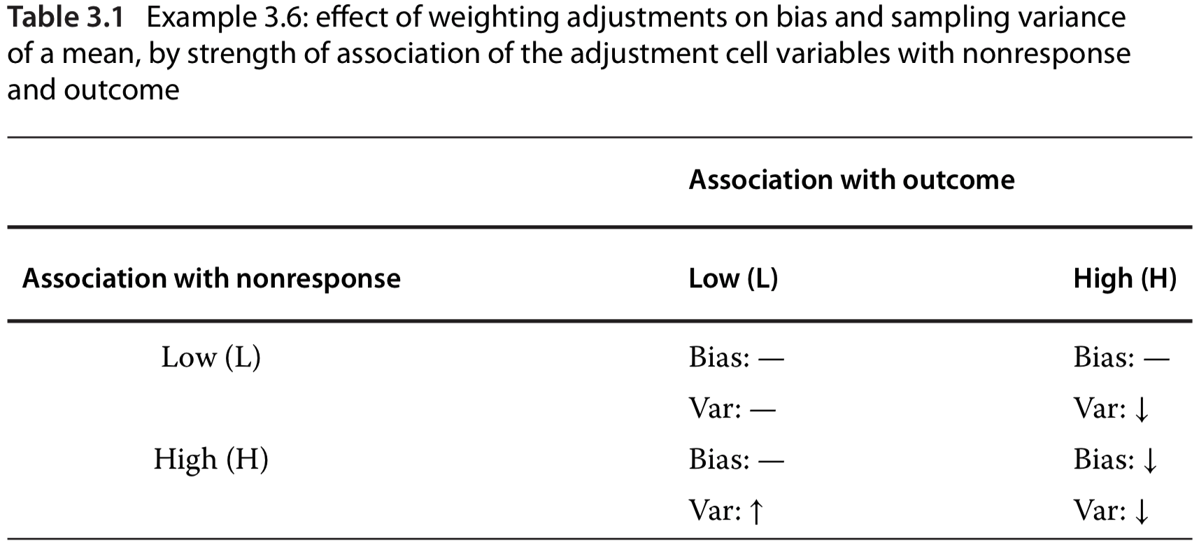
Cons: weighting is inefficient and can increase in sampling variance, if $Y$ is weakly related to the weighting class variable $C$

How to choose weighting class adjustments: weighting is only effective for outcomes ($Y$) that are associated with the adjustment cell variable ($C$). See the right column in the table below.

The theory of propensity scores provides a prescription for choosing the coarsest reduction of $X$ to a weighting class variable $C$ so that quasirandomization is roughly satisfied

Let $X$ denote the variables observed for both respondents and nonrespondents

Suppose data are MAR, with $\varphi$ being unknown parameters about missing mechanism $$P(M\mid X,Y,\varphi )=P(M\mid X,\varphi )$$ Then quasirandomization is satisfied when $C$ is chosen to be $X$

Define response propensity for unit $i$ as $$\rho (x_i,\varphi )=P(m_i=0\mid \rho (x_i,\varphi ),\varphi )$$ i.e., respondents are a random subsample within strata defined by the propensity score $\rho (X,\varphi )$

Usually $\varphi$ is unknown. So a practical procedure is

1. Estimate $\hat{\varphi }$ from a binary regression of $M$ on $X$, based on respondent and nonrespondent data
2. Let $C$ be a grouped variable by coarsening $\rho (X,\hat{\varphi })$ into 5 or 10 values

Thus, within the same adjustment class, all respondents and nonrespondents have the same value of the grouped propensity score

An alternative procedure is to weight respondents $i$ directly by the inverse propensity score $\rho {(X,\hat{\varphi })}^{-1}$

This method removes nonresponse bias

But it may yield estimates with extremely high sampling variance because respondents with very low estimated response propensities receive large nonresponse weights

Also, weighting directly by inverse propensities place may reliance on correct model specification of the regression of $M$ on $X$

Let $x_i$ be covariates of GEE, and $z_i$ be a fully observed vector that can predict missing mechanism

If $P(m_i=1\mid x_i,y_i,z_i,\varphi )=P(m_i=1\mid x_i,\varphi )$, then the unweighted completed case GEE is unbiased $$\sum _{i=1}^r{D}_i(x_i,\beta )[y_i-g(x_i,\beta \left)\right]=0$$

If $P(m_i=1\mid x_i,y_i,z_i,\varphi )=P(m_i=1\mid x_i,z_i,\varphi )$, then the inverse probability weighted GEE is unbiased $$\sum _{i=1}^r{w}_i\left(\hat{\alpha }\right)D_i(x_i,\beta )[y_i-g(x_i,\beta \left)\right]=0,w_i\left(\hat{\alpha }\right)=\frac{1}{p(x_i,z_i\mid \hat{\alpha })}$$ where $p(x_i,z_i\mid \hat{\alpha })$ is the probability of being a complete unit, based on logistic regression of $m_i$ on $x_i,z_i$

The weighting class estimator $${\overline{y}}_{\text{wc}}=\frac{1}{n}\sum _{j=1}^J{n}_j{\overline{y}}_{j\text{R}}$$ uses the sample proportion $n_j/n$ to estimate the population proportion $N_j/N$.

If from an external resource (e.g., census or a large survey), we know the population proportion of weighting classes, then we can use the post stratified mean to estimate $\overline{Y}$: $${\overline{y}}_{\text{ps}}=\frac{1}{N}\sum _{j=1}^J{N}_j{\overline{y}}_{j\text{R}}$$

Weighted CC estimates are often simple to compute, but the appropriate standard errors can be hard to compute (even asymptotically)

Weighting methods treat weights as fixed and known, but these nonresponse weights are computed from observed data and hence are subject to sampling uncertainty

Because weighted CC methods discard incomplete units and do not provide an automatic control of sampling variance, they are most useful when

• Number of covariates is small, and
• Sample size is large

Available-case analysis: for univariate analysis, include all unites where that variable is present

• Sample changes from variable to variable according to the pattern of missing data
• This is problematic if not MCAR
• Under MCAR, AC can be used to estimate mean and variance for a single variable

Pairwise AC: estimates covariance of $Y_j$ and $Y_k$ based on units $i$ where both $y_{ij}$ and $y_{ik}$ are observed

• Pairwise covariance estimator: $$s_{jk}^{\left(jk\right)}=\sum _{i\in I_{jk}}(y_{ij}-{\overline{y}}_j^{\left(jk\right)})(y_{ik}-{\overline{y}}_k^{\left(jk\right)})/(n^{\left(jk\right)}-1)$$ where $I_{jk}$ is the set of $n^{\left(jk\right)}$ units with both $Y_j$ and $Y_k$ observed

Correlation estimator 1: $$r_{jk}^{\ast }=\frac{s_{jk}^{\left(jk\right)}}{\sqrt{s_{jj}^{\left(j\right)}{s}_{kk}^{\left(k\right)}}}$$

• Problem: it can lie outside of $(-1,1)$

Correlation estimator 2 corrects the previous problem: $$r_{jk}^{\left(jk\right)}=\frac{s_{jk}^{\left(jk\right)}}{\sqrt{s_{jj}^{\left(jk\right)}{s}_{kk}^{\left(jk\right)}}}$$

Under MCAR, all these estimators on covariance and correlation are consistent

However, when $K>3$, both correlation estimators can yield correlation matrices that are not positive definite!

• An extreme example: $r_{12}=1,r_{13}=1,r_{23}=-1$

When data is MCAR and correlations are mild, AC methods are more efficient than CC

When correlations are large, CC methods are usually better

References

- Little, R. J., & Rubin, D. B. (2019). Statistical Analysis with Missing Data, 3rd Edition. John Wiley & Sons.