For the pdf slides, click here
Ch1 Introduction
Three most common types of NNs in NLP
Feed-forward networks, i.e., multi-layer perceptrons (MLPs), or fully connected layers
- Allow to work with fixed sized inputs
- Or with variable length inputs in which we can disregard the order of the elements (continuous bags of words)
Recurrent neural networks (RNNs)
- Specialized models for sequential data
- Produce a fixed size vector that summarizes the sequence
- Doesn’t require fixed sized input (e.g., lengths of input sequence can vary)
Convolutional feed-forward networks (CNNs)
- Good at extracting local patterns in the data
About neural networks
Some of the neural network techniques (e.g., MLP) are simple generalizations of the linear models and can be used as almost drop-in replacements for the linear classifiers
RNNs and CNNs are rarely used as standalone components. They are used to extract features and being fed into other network components, and trained to work in tandem with them.
Success stories
Multi-layer feed-forward networks can provide competitive results on sentiment classification and factoid question answering
Networks with convolutional and pooling layers are useful for classification tasks in which we expect to find strong local clues regarding class membership, but these clues can appear in different places in the input
- Convolutional and pooling layers allow the model to learn to find such local indicators, regardless of their position
Note
- In this book, vectors are assumed to be row vectors
Ch2 Linear Models
One-hot and dense vector representations (p23)
The input \(\mathbf{x}\) in language classification example contains the normalized bigram counts in the document \(D\)
- \(D_{[i]}\) is the bigram at document position \(i\)
Each vector \(\mathbf{x}^{D_{[i]}} \in \mathbb{R}^{d}\) is a one-hot vector
The following \(\mathbf{x}\) is an averaged bag of words, or just bag of words: \[ \mathbf{x} = \frac{1}{|D|} \sum_{i=1}^{|D|} \mathbf{x}^{D_{[i]}} \]
Bag of words doesn’t consider orders among words
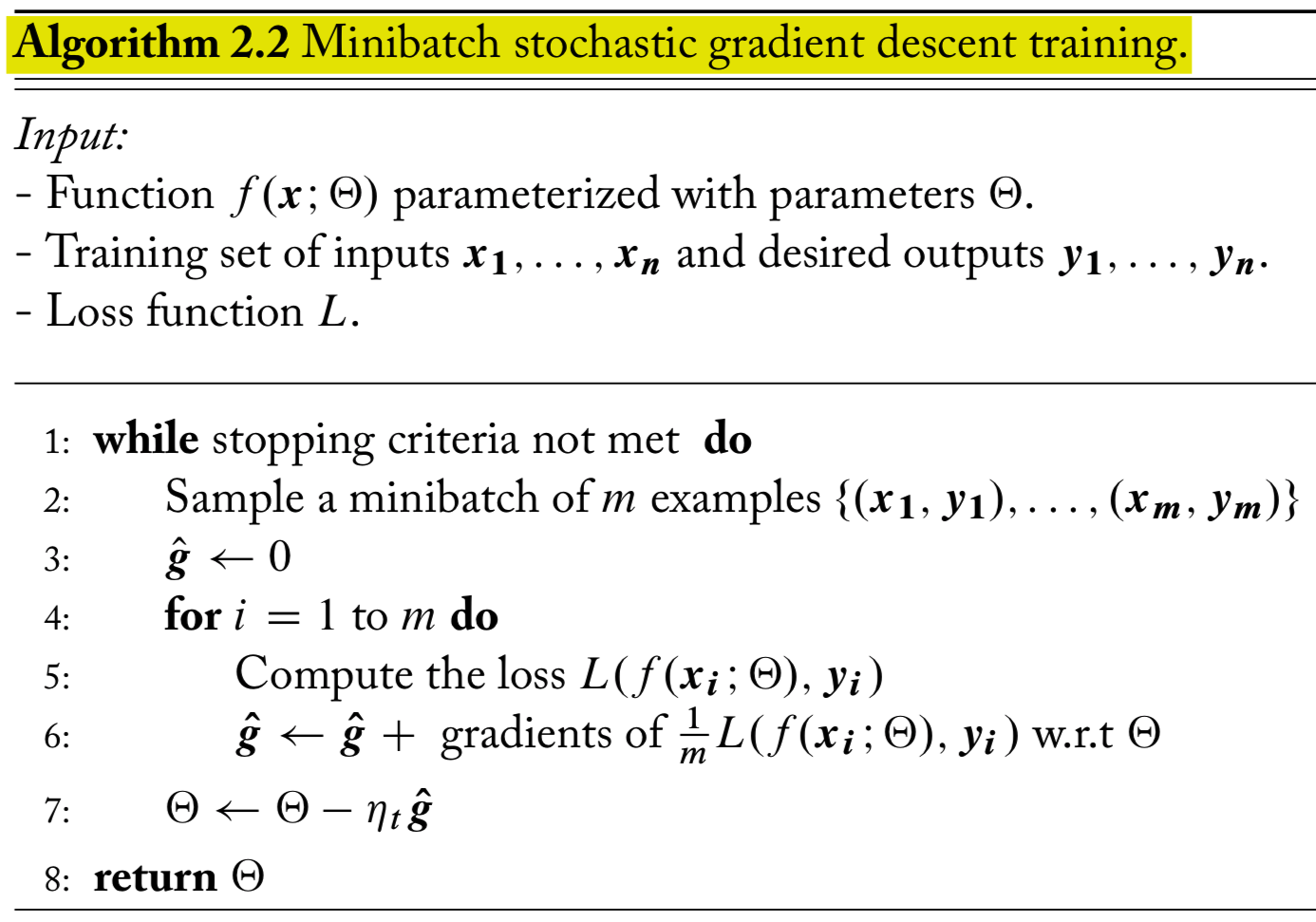
Minibatch stochastic gradient descent (SGD) algorithm (p32)
Goal: set the parameters \(\Theta\) to minimize the total loss \[ \mathcal{L}(\Theta) = \sum_{i=1}^n L\left(f(\mathbf{x}_i; \theta), \mathbf{y}_i \right) \] over the training set
Learning rate: \(\eta_t\)
Minibatch size \(m\), can vary from \(m=1\) to \(m=n\)
After the inner loop, \(\hat{\mathbf{g}}\) contains the gradient estimate
Ch4 Feed-Forward Neural Networks

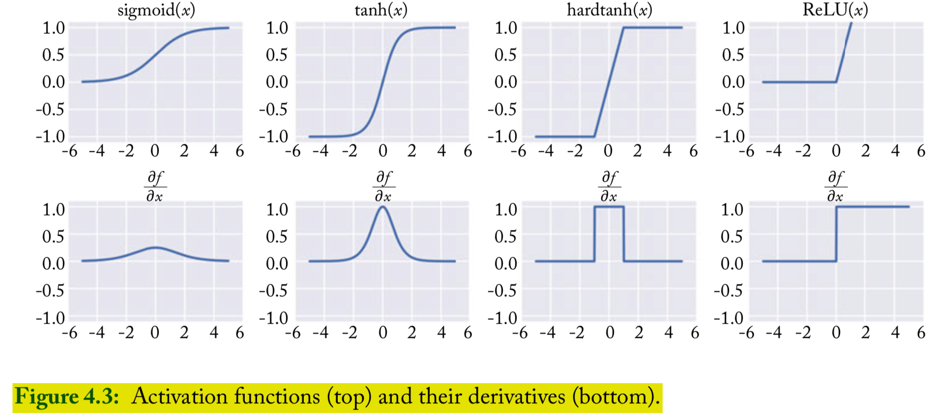
Common nonlinearities (p45)
Sigmoid (currently considered to be deprecated for use in internal layers of NN)
Hyperbolic tangent (tanh): common
ReLU: common
Regularization and dropout
L2 regularization, also called weight decay is effective, and tuning the regularization strength \(\lambda\) is advisable
Dropout training: randomly dropping (setting to zero) half of the neurons in the network in each training example in the stochastic-gradient training
Dropout is effective in NLP applications of NNs
Ch5 Neural Network Training
Comment
The objective function for nonlinear neural networks is not convex, and gradient-based methods may get stuck in a local minima
Still, gradient-based methods produce good results in practice
Choice of optimization algorithm: the book author likes Adam, as it is very effective and relatively robust to the choice of learning rate
Initialization
It is advised to run several restarts of the training starting at different random initializations, and choosing the best one based on a development set
Xavier initialization:
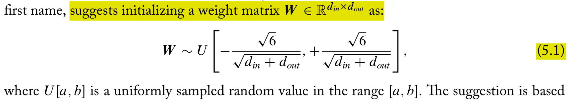
When using ReLU nonlinearities, the following Gaussian initialization may work better than Xavier. The weights should be initialized by sampling from a zero-mean Gaussian distribution whose sd is \(\sqrt{2/d_{\text{in}}}\)
Vanishing and exploding gradients
Vanishing gradients
batch-normalization, i.e., for every minibatch, normalize the inputs to each of the network layers to have zero mean and unit variance
Or use specialized architectures that are designed to assist in gradient flow (i.e., LSTM and GRU)
Exploding gradients: clipping the gradients if their norm exceeds a given threshold
Learning rate
Experiment with a range of initial learning rates in range \([0, 1]\), e.g., 0.001, 0.01, 0.1, 1.
Learning rate scheduling decreases the rate as a function of the number of observed minibatches
A common schedule is dividing the initial learning rate by the iteration number
Bottou’s recommendation: \[ \eta_t = \frac{\eta_0}{1 + \eta_0 \lambda t} \]
References
- Goldberg, Yoav. (2017). Neural Network Methods for Natural Language Processing, Morgan & Claypool