For the pdf slides, click here
Overview of Gaussian processes (GP)
The problem is learning in GP is exactly the problem of finding suitable properties for the covariance function
In this book, design matrix is defined slightly differently from common statistical textbooks. Rather, each column in a design matrix is a case, and each row is a covariate
Weight-space View
A regression model with basis functions
Basis function \(\boldsymbol\phi(\mathbf{x})\): maps a \(D\)-dimensional input vector \(\mathbf{x}\) into an \(N\)-dimensional feature space
\(\boldsymbol\Phi(\mathbf{X}) \in \mathbb{R}^{N \times n}\): the aggregation of columns \(\boldsymbol\phi(\mathbf{x})\) for all \(n\) cases in the training data
A regression model \[ f(\mathbf{x}) = \boldsymbol\phi(\mathbf{x})^\top \mathbf{w}, \quad y = f(\mathbf{x}) + \epsilon, \quad \epsilon \sim \mathcal{N}(0, \sigma^2_n) \]
We use a zero mean Gaussian prior on the \(N\)-dimensional unknown weights \(\mathbf{w}\) (aka regression coefficients) \[ \mathbf{w} \sim \mathcal{N}(\mathbf{0}, \boldsymbol\Sigma_p) \]
Predictive distribution
For a new test point \(\mathbf{x}_*\), the predictive distribution is \[\begin{align*} f_* \mid \mathbf{x}_*, \mathbf{X}, \mathbf{y} & \sim \mathcal{N}\left(\frac{1}{\sigma^2_n} \boldsymbol\phi_*^\top \mathbf{A}^{-1}\boldsymbol\Phi \mathbf{y},\quad \boldsymbol\phi_*^\top \mathbf{A}^{-1} \boldsymbol\phi_* \right),\\ \boldsymbol\phi_* &= \boldsymbol\phi(\mathbf{x}_*), \quad \boldsymbol\Phi = \boldsymbol\Phi(\mathbf{X}), \quad \mathbf{A} = \frac{1}{\sigma^2_n} \boldsymbol\Phi \boldsymbol\Phi^\top + \boldsymbol\Sigma_p^{-1} \end{align*}\]
When make predictions, we need to invert the \(N\times N\) matrix \(\mathbf{A}\), which may not be convenient if \(N\), the dimension of the feature space, is large
Rewriting the predictive distribution using the matrix inversion lemma
Marix inversion lemma: \(\mathbf{Z} \in \mathbb{R}^{n \times n}\), \(\mathbf{W} \in \mathbb{R}^{m \times m}\), \(\mathbf{U}, \mathbf{V}\in \mathbb{R}^{n \times m}\) \[ \left( \mathbf{Z} + \mathbf{U} \mathbf{W} \mathbf{V}^\top \right)^{-1} = \mathbf{Z}^{-1} - \mathbf{Z}^{-1} \mathbf{U} \left( \mathbf{W}^{-1} + \mathbf{V}^\top \mathbf{Z}^{-1} \mathbf{U}\right)^{-1} \mathbf{V}^\top\mathbf{Z}^{-1} \]
We can rewrite the predictive distribution on the previous page as \[\begin{align}\label{eq:weight_space_prediction} f_* \mid \mathbf{x}_*, \mathbf{X}, \mathbf{y} & \sim \mathcal{N}\left( \boldsymbol\phi_*^\top \boldsymbol\Sigma_p \boldsymbol\Phi \left(\mathbf{K} + \sigma^2_n \mathbf{I} \right)^{-1}\mathbf{y}, \right.\\ \nonumber & ~~~~~~~~~\left. \boldsymbol\phi_*^\top \boldsymbol\Sigma_p \boldsymbol\phi_* - \boldsymbol\phi_*^\top \boldsymbol\Sigma_p \boldsymbol\Phi \left(\mathbf{K} + \sigma^2_n \mathbf{I} \right)^{-1} \boldsymbol\Phi^\top \boldsymbol\Sigma_p \boldsymbol\phi_* \right),\\ \nonumber \mathbf{K} &= \boldsymbol\Phi^\top \boldsymbol\Sigma_p \boldsymbol\Phi \end{align}\]
Kernel and the kernel trick
In the predictive distribution on the previous page, the feature space always enters in the form of the kernel \(k(\cdot, \cdot)\): \[ k(\mathbf{x}, \mathbf{x}^\prime) = \boldsymbol\phi(\mathbf{x})^\top\boldsymbol\Sigma_p \boldsymbol\phi(\mathbf{x}^\prime), \] where \(\mathbf{x}, \mathbf{x}^\prime\) are in either the training or the test sets
Moreover, we can define \[ \boldsymbol\psi(\mathbf{x}) = \boldsymbol\Sigma_p^{1/2} \boldsymbol\phi(\mathbf{x}), \] so that the kernel has a simple dot product representation \[ k(\mathbf{x}, \mathbf{x}^\prime) = \boldsymbol\psi(\mathbf{x}) \cdot \boldsymbol\psi(\mathbf{x}^\prime) \]
Kernel trick: if an algorithm is defined solely in terms of inner products in input space, the it can be lifted into feature space by replacing occurrences of those inner products by \(k(\mathbf{x}, \mathbf{x}^\prime)\)
Function-space View
Gaussian process: definition
A Gaussian process(GP) is a collection of random variables, any finite number of which have a joint Gaussian distribution
A GP is completely specified by its mean function \(m(\mathbf{x})\) and covariance function \(k(\mathbf{x}, \mathbf{x}^\prime)\) \[ f(\mathbf{x}) \sim \mathcal{GP}\left(m(\mathbf{x}), k(\mathbf{x}, \mathbf{x}^\prime) \right) \]
Usually the prior mean function is set to zero
Bayesian linear regression as a Gaussian process \[ f(\mathbf{x}) = \boldsymbol\phi(\mathbf{x})^\top \mathbf{w}, \quad \mathbf{w} \sim \mathcal{N}(\mathbf{0}, \boldsymbol\Sigma_p) \] Here, the GP mean function and the covariance function are \[ m(\mathbf{x}) = \mathbf{0}, \quad k(\mathbf{x}, \mathbf{x}^\prime) = \boldsymbol\phi(\mathbf{x})^\top \boldsymbol\Sigma_p \boldsymbol\phi(\mathbf{x}^\prime) \]
The squared exponential covariance function
In this chapter, squared exponential (SE) covariance function will be used \[ \text{cov}\left(f(\mathbf{x}), f(\mathbf{x}^\prime) \right) = k(\mathbf{x}, \mathbf{x}^\prime) = \exp\left(-\frac{1}{2}\left|\mathbf{x}- \mathbf{x}^\prime \right|^2 \right) \]
By replacing \(\left|\mathbf{x}- \mathbf{x}^\prime \right|\) by \(\left|\mathbf{x}- \mathbf{x}^\prime \right|/\ell\) for some positive constant \(\ell\), we can change the characteristic length-scale of the process
Note that the covariance between the outputs is written as a function of the inputs
The squared exponential covariance function corresponds to a Bayesian linear regression model with a infinite number of basis functions
Actually for every positive definite covariance function \(k(\cdot, \cdot)\), there exists a (possibly infinite) expansion in terms of basis functions
Three functions drawn at random from a GP prior (left) and their posteriors (right)
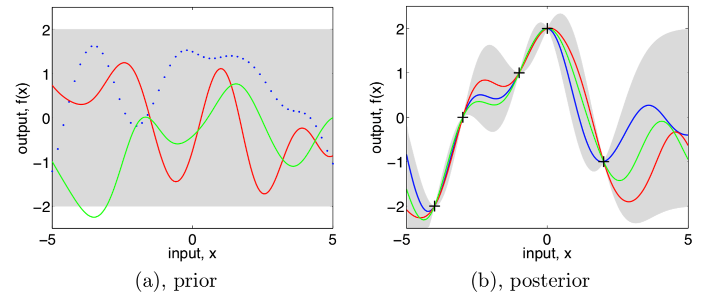
- In both plots, shaded area are the pointwise mean plus and minus two times the standard deviation from each input value
Prediction with noise-free observations
Prediction with noise-free observations
Suppose we have noise-free observations \(\{\left(\mathbf{x}_i, f_i\right): i = 1, \ldots, n\}\)
According to the GP prior, the joint distribution of the training outputs \(\mathbf{f}\) and the test outputs \(\mathbf{f}_*\) is \[ \left[ \begin{array}{l} \mathbf{f}\\ \mathbf{f}_* \end{array} \right] \sim \mathcal{N}\left(\mathbf{0}, \left[ \begin{array}{ll} K(\mathbf{X}, \mathbf{X}) & K(\mathbf{X}, \mathbf{X}_*)\\ K(\mathbf{X}_*, \mathbf{X}) & K(\mathbf{X}_*, \mathbf{X}_*) \end{array} \right] \right) \]
By conditioning the joint Gaussian prior on the observations, we get the posterior distribution \[\begin{align*} \mathbf{f}_* \mid \mathbf{X}_*, \mathbf{X}, \mathbf{f} &\sim \mathcal{N}\left( K(\mathbf{X}_*, \mathbf{X}) K(\mathbf{X}, \mathbf{X})^{-1} \mathbf{f}, \right.\\ &~~~~~~~~~~\left. K(\mathbf{X}_*, \mathbf{X}_*) - K(\mathbf{X}_*, \mathbf{X}) K(\mathbf{X}, \mathbf{X})^{-1}K(\mathbf{X}, \mathbf{X}_*) \right) \end{align*}\]
Prediction with noisy observations
Prediction with noisy observations
With noisy observations \(y = f(\mathbf{x}) + \epsilon\), the covariance becomes \[ \text{cov}(\mathbf{y}) = K(\mathbf{X}, \mathbf{X}) + \sigma^2_n \mathbf{I} \]
Thus, the joint prior distribution becomes \[ \left[ \begin{array}{l} \mathbf{y}\\ \mathbf{f}_* \end{array} \right] \sim \mathcal{N}\left(\mathbf{0}, \left[ \begin{array}{cc} K(\mathbf{X}, \mathbf{X}) + \sigma^2_n \mathbf{I} & K(\mathbf{X}, \mathbf{X}_*)\\ K(\mathbf{X}_*, \mathbf{X}) & K(\mathbf{X}_*, \mathbf{X}_*) \end{array} \right] \right) \]
Key predictive equation for GP regression \[\begin{align}\label{eq:function_space_prediction} \mathbf{f}_* \mid \mathbf{X}_*, \mathbf{X}, \mathbf{f} &\sim \mathcal{N}\left( \bar{\mathbf{f}}_*, \text{cov}(\mathbf{f}_*)\right), \quad \text{where}\\ \nonumber \bar{\mathbf{f}}_* & = K(\mathbf{X}_*, \mathbf{X}) \left[K(\mathbf{X}, \mathbf{X})+ \sigma^2_n\right]^{-1} \mathbf{y}\\ \nonumber \text{cov}(\mathbf{f}_*) & = K(\mathbf{X}_*, \mathbf{X}_*) - K(\mathbf{X}_*, \mathbf{X}) \left[K(\mathbf{X}, \mathbf{X})+ \sigma^2_n\right]^{-1}K(\mathbf{X}, \mathbf{X}_*) \end{align}\]
Correspondence with weight-space view
Connection between the function-space view, Eq , and the weight-space view, Eq \[ K(C, D) = \boldsymbol\Phi(C)^\top \boldsymbol\Sigma_p \boldsymbol\Phi(D) \] where \(C, D\) stand for either \(\mathbf{X}\) or \(\mathbf{X}_*\)
Thus, for any set of basic functions, we can compute the corresponding covariance function as \[ k(\mathbf{x}, \mathbf{x}^\prime) = \boldsymbol\phi(\mathbf{x})^\top \boldsymbol\Sigma_p \boldsymbol\phi(\mathbf{x}^\prime) \]
On the other hand, for every positive definite covariance function \(k\), there exists a possibly infinite expansion in terms of basis functions
Predictive distribution for a single test point \(\mathbf{x}_*\)
- Denote \(K = K(\mathbf{X}, \mathbf{X})\) and \(\mathbf{k}_* = K(\mathbf{X}, \mathbf{x}_*)\), then the mean and variance of the posterior predictive distribution are \[\begin{align}\label{eq:predictive_mean} \bar{\mathbf{f}}_* & = \mathbf{k}_*^\top\left(K + \sigma^2_n \mathbf{I} \right)^{-1}\mathbf{y},\\ \label{eq:predictive_covariance} \mathbb{V}(\mathbf{f}_*) & = k(\mathbf{x}_*, \mathbf{x}_*) - \mathbf{k}_*^\top\left(K + \sigma^2_n \mathbf{I} \right)^{-1}\mathbf{k}_* \end{align}\]
Predictive distribution mean as a linear predictor
The mean prediction Eq is a linear predictor, i.e., it’s a linear combination of observations \(\mathbf{y}\)
Another way to look at this equation is to see it as a linear combination of \(n\) kernel functions \[ \bar{f}(\mathbf{x}_*) = \sum_{i=1}^n \alpha_i k(\mathbf{x}_i, \mathbf{x}_*), \quad \boldsymbol\alpha = \left(K + \sigma^2_n \mathbf{I} \right)^{-1}\mathbf{y} \]
About the predictive distribution variance
The predictive variance Eq does not depend on the observed targets \(\mathbf{y}\), but only the inputs. This is a property of the Gaussian distribution
The noisy prediction of \(\mathbf{y}_*\): simply add \(\sigma^2_n \mathbf{I}\) to the variance \[ \mathbf{y}_* \mid \mathbf{x}_*, \mathbf{X}, \mathbf{y} \sim \mathcal{N} \left(\bar{\mathbf{f}}_*, \mathbb{V}(\mathbf{f}_*) + \sigma^2_n \mathbf{I} \right) \]
Cholesky decomposition and GP regression algorithm
Cholesky decomposition
Cholesky decomposition of a symmetric, positive definite matrix \(\mathbf{A}\) \[ \mathbf{A} = \mathbf{L}\mathbf{L}^\top, \] where \(\mathbf{L}\) is a lower triangular matrix, called the Cholesky factor
- Cholesky decomposition is useful for solving linear systems with symmetric, positive definite coefficient matrix: to solve \(\mathbf{A}\mathbf{x} = \mathbf{b}\)
- First solve the triangular system \(\mathbf{L}\mathbf{y} = \mathbf{b}\) by forward substitution
- Then the triangular system \(\mathbf{L}^\top\mathbf{x} = \mathbf{y}\) by back substitution
Backslash operator: \(\mathbf{A}\backslash\mathbf{b}\) is the vector \(\mathbf{x}\) which solves \(\mathbf{A}\mathbf{x} = \mathbf{b}\)
- Under Cholesky decomposition, \[ \mathbf{x} = \mathbf{A}\backslash\mathbf{b} = \mathbf{L}^\top \backslash \left( \mathbf{L} \backslash \mathbf{b}\right) \]
The computation of the Cholesky factor \(\mathbf{L}\) is considered numerically extremely stable, and takes time’ \(n^3/6\)
Algorithm: predictions and log marginal likelihood for GP regression
- Input: \(\mathbf{X}, \mathbf{y}, k, \sigma^2_n, \mathbf{x}_*\)
\(\mathbf{L} = \text{cholesky} \left(K + \sigma^2_n \mathbf{I} \right)\)
\(\boldsymbol\alpha = \mathbf{L}^\top \backslash \left( \mathbf{L} \backslash \mathbf{y}\right)\)
\(\bar{f}_* = \mathbf{k}_*^\top \boldsymbol\alpha\)
\(\mathbf{v} = \mathbf{L} \backslash \mathbf{k}_*\)
\(\mathbb{V}(\mathbf{f}_*) = k(\mathbf{x}_*, \mathbf{x}_*) - \mathbf{v}^\top \mathbf{v}\)
\(\log p(\mathbf{y}\mid \mathbf{X}) = -\frac{1}{2}\mathbf{y}^\top \boldsymbol\alpha - \sum_i \log L_{ii} - \frac{n}{2}\log 2\pi\)
Return: \(\bar{f}_*, \mathbb{V}(\mathbf{f}_*), \log p(\mathbf{y}\mid \mathbf{X})\)
Computational complexity: \(n^3/6\) for the Cholesky decomposition in Line 1, and \(n^2/2\) for solving triangular systems in Line 2, 4
Hyperparameters
Hyperparameters
One-dimensional squared-exponential covariance function \[ k_y(x_p, x_q) = \sigma^2_f \exp\left[ -\frac{1}{2\ell^2}(x_p - x_q)^2 \right] + \sigma^2_n \delta_{pq} \]
- It has three hyperparameters
- Length-scale \(\ell\)
- Signal variance \(\sigma^2_f\)
- Noise variance \(\sigma^2_n\)
After selected \(\ell\), the rest two hyperparameters are set by optimizing the marginal likelihood \[ \log p(\mathbf{y}\mid \mathbf{X}) = -\frac{1}{2}\mathbf{y}^\top \left(K + \sigma^2_n \mathbf{I} \right)^{-1}\mathbf{y} - \frac{1}{2}\log \left| K + \sigma^2_n \mathbf{I} \right| - \frac{n}{2}\log 2\pi \]
Smoothing, Weight Functions, and Equivalent Kernels
TO BE CONTINUED
References
Rasmussen, C. E. and Williams, C. K. I. (2006). Gaussian Processes for Machine learning, MIT press.