Exponential family of distributions

• The density function for an exponential family distribution \[\begin{equation}\label{eq:exponential_family_density} f(y) = \exp\left\{ \frac{y\theta - b(\theta)}{a(\phi)} + c(y, \phi) \right\} \end{equation}\]
  • \(a, b, c\): arbitrary functions
  • \(\phi\): an arbitrary scale parameter
  • \(\theta\): the canonical parameter; completely depend on the model parameter \(\boldsymbol\beta\)

• Properties about exponential family mean and variance \[\begin{align*} E(Y) & = b^{\prime}(\theta)\\ var(Y) & = b^{\prime\prime}(\theta) a(\phi) \end{align*}\]

  • In most practical cases, \(a(\phi) = \phi/\omega\) where \(\omega\) is a known constant
  • We define a function \[ V(\mu) = b^{\prime\prime}(\theta) / w, \quad \text{so that } var(Y) = V(\mu) \phi \]

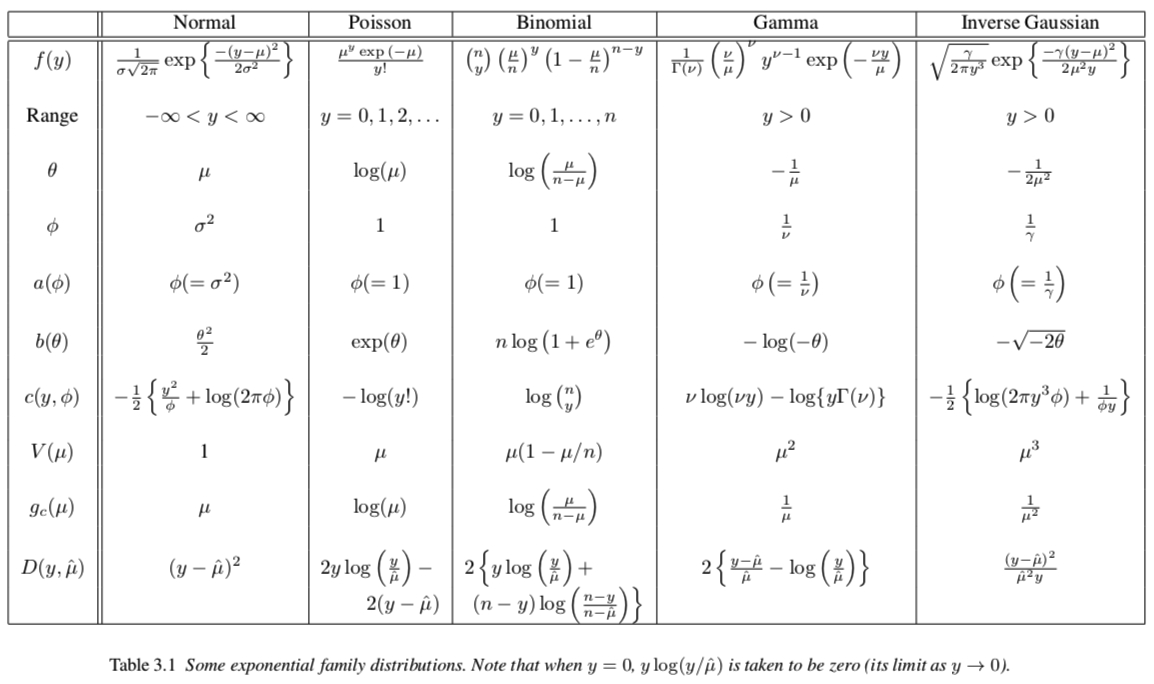
Exponential family examples

Fitting GLMs

• For the GLM model and , assuming \(a_i(\phi) = \phi/\omega_i\), the log likelihood is \[ l(\boldsymbol\beta) = \sum_{i=1}^n \omega_i \left[ y_i \theta_i - b_i(\theta_i) \right]/\phi + c_i(\phi, y_i) \]

• To optimize, we use the Newton’s method, which is an iterative optimization approach \[ \theta^{(t+1)} = \theta^{(t)} - \left(\nabla^2 l\right)^{-1}\nabla l \]
  • Where both \(\nabla^2 l\) and \(\nabla l\) are evaluated at the current iteration \(\theta^{(t)}\)
  • Alternatively, we can use the Fisher scoring variant of the Newton’s method, by replacing the Hessian matrix with its expectation

• Next, we will need to compute the gradient vector and expected Hessian matrix of \(l\)

Compute the gradient vector and expected Hessian of \(l\)

• By the chain rule, \[\begin{align*} \frac{\partial \theta_i}{\partial \beta_j} & = \frac{\partial \theta_i}{\partial \mu_i} \cdot \frac{\partial \mu_i}{\partial \eta_i} \cdot \frac{\partial \eta_i}{\partial \beta_j} \\ & = \frac{1}{b^{\prime\prime}(\theta_i)}\cdot \frac{1}{g^{\prime}(\mu_i)}\cdot X_{ij} \end{align*}\]

• Therefore, the gradient vector of \(l\) is \[\begin{align*} \frac{\partial l}{\partial \beta_j} = \frac{1}{\phi} \sum_{i=1}^n \omega_i \left[y_i - b^{\prime}_i(\theta_i) \right]\frac{\partial \theta_i}{\partial \beta_j} = \frac{1}{\phi}\sum_{i=1}^n \frac{y_i - \mu_i}{g^{\prime}(\mu_i) V(\mu_i)} X_{ij} \end{align*}\]

• The expected Hessian (expectation taken wrt \(Y\)) is \[ E\left( \frac{\partial^2 l}{\partial \beta_j \partial \beta_k} \right) = - \frac{1}{\phi}\sum_{i=1}^n \frac{X_{ij} X_{ik}}{g^{\prime}(\mu_i)^2 V(\mu_i)} \]

The Fisher scoring update

• Define the matrices \[\begin{align}\label{eq:W} \mathbf{W} & = \text{diag}\{w_i\}, \quad w_i = \frac{1}{g^{\prime}(\mu_i)^2 V(\mu_i)} \\ \label{eq:G} \mathbf{G} & = \text{diag}\left\{g^{\prime}(\mu_i)\right\} \end{align}\]

• The Fisher scoring update for \(\boldsymbol\beta\) is \[\begin{align*} \boldsymbol\beta^{(t+1)} & = \boldsymbol\beta^{(t)} + \left(\mathbf{X}^T \mathbf{W} \mathbf{X} \right)^{-1} \mathbf{X}^T \mathbf{W} \mathbf{G} (\mathbf{y} - \boldsymbol\mu)\\ & = \left(\mathbf{X}^T \mathbf{W} \mathbf{X} \right)^{-1} \mathbf{X}^T \mathbf{W} \underbrace{\left[ \mathbf{G}(\mathbf{y} - \boldsymbol\mu) + \mathbf{X}\boldsymbol\beta^{(t)} \right]}_{\mathbf{z}} \end{align*}\]

Iteratively re-weighted least square (IRLS) algorithm

1. Initialization: \[ \hat{\mu}_i = y_i + \delta_i, \quad \hat{\eta}_i = g\left(\hat{\mu}_i\right) \]

   • \(\delta_i\) is usually zero, but may be a small constant ensuring \(\hat{\eta}_i\) is finite

2. Compute pseudo data \(z_i\) and iterative weights \(w_i\): \[\begin{align*} z_i &= g^{\prime}\left(\hat{\mu}_i\right)\left(y_i - \hat{\mu}_i\right) + \hat{\eta}_i\\ w_i &= \frac{1}{g^{\prime}\left(\hat{\mu}_i\right)^2 V\left(\hat{\mu}_i\right)} \end{align*}\]

3. Find \(\hat{\boldsymbol\beta}\) by minimizing the weighted least squares objective \[ \sum_{i=1}^n w_i \left(z_i -\mathbf{X}_i \boldsymbol\beta \right)^2 \] then update \[ \hat{\boldsymbol\eta} = \mathbf{X} \hat{\boldsymbol\beta}, \quad \hat{\mu}_i = g^{-1}\left(\hat{\eta}_i\right) \]

• Repeat Step 2-3 until the change in deviance is near zero

IRLS example 1: logistic regression

• For logistic regression, \[\begin{align*} g(\mu) & = \log\left(\frac{\mu}{1 - \mu}\right), \quad g^{\prime}(\mu) = \frac{1}{\mu (1-\mu)}\\ V(\mu) &= \mu (1-\mu), \quad\quad\quad \phi =1 \end{align*}\]

• Therefore, in Step 2 of IRLS, \[\begin{align*} z_i & = \frac{y_i - \hat{\mu}_i}{\hat{\mu}_i\left(1-\hat{\mu}_i\right)} + \hat{\eta}_i \\ w_i & = \hat{\mu}_i\left(1-\hat{\mu}_i\right) \end{align*}\]

IRLS example 2: GLM with independent normal priors

• Assume that the vector \(\boldsymbol\beta\) has independent normal priors \[ \boldsymbol\beta \sim \text{N}\left(\mathbf{0}, \frac{\phi}{\lambda}\mathbf{I}_p \right) \]

• Log posterior density (we still call it \(l\), with some abuse of notation) \[ l(\boldsymbol\beta) = \frac{1}{\phi}\sum_{i=1}^n \omega_i \left[ y_i \theta_i - b_i(\theta_i) \right]- \frac{\lambda}{2\phi}\boldsymbol\beta^T \boldsymbol\beta + \text{const} \]

• Gradient vector and expected Hessian matrix (wrt \(\boldsymbol\beta\)) \[\begin{align*} \nabla l &= \frac{1}{\phi} \left[\mathbf{X}^T \mathbf{W}\mathbf{G}(\mathbf{y} - \boldsymbol\mu) - \lambda \boldsymbol\beta\right]\\ E\left(\nabla^2 l \right) &= -\frac{1}{\phi}\left(\mathbf{X}^T \mathbf{W}\mathbf{X} + \lambda \mathbf{I}_p \right) \end{align*}\]

  • Here, \(\mathbf{W}\) and \(\mathbf{G}\) are the same as in Equation and

• IRLS for GLM with independent normal priors \[\begin{align}\notag \boldsymbol\beta^{(t+1)} & = \boldsymbol\beta^{(t)} + \left(\mathbf{X}^T \mathbf{W} \mathbf{X} + \lambda \mathbf{I}_p \right)^{-1} \left[\mathbf{X}^T \mathbf{W} \mathbf{G}(\mathbf{y} - \boldsymbol\mu) - \lambda \boldsymbol\beta^{(t)}\right] \\ \label{eq:IRLS_penalty} & = \left(\mathbf{X}^T \mathbf{W} \mathbf{X} + \lambda \mathbf{I}_p\right)^{-1} \mathbf{X}^T \mathbf{W} \underbrace{\left[ \mathbf{G}(\mathbf{y} - \boldsymbol\mu) + \mathbf{X}\boldsymbol\beta^{(t)} \right]}_{\mathbf{z}} \end{align}\]

Large sample distribution of \(\hat{\boldsymbol\beta}\)

• Hessian of the negative log likelihood (also called observed information) \[ \hat{\mathcal{I}} = \frac{\mathbf{X}^T \mathbf{W} \mathbf{X}}{\phi} \]

• Fisher information, also called expected information \[ \mathcal{I} = E\left(\hat{\mathcal{I}}\right) \]

• Asymptotic normality the MLE \(\hat{\boldsymbol\beta}\) \[ \hat{\boldsymbol\beta} \sim \text{N}\left(\boldsymbol\beta, \mathcal{I}^{-1} \right) \quad \text{or} \quad \hat{\boldsymbol\beta} \sim \text{N}\left(\boldsymbol\beta, \hat{\mathcal{I}}^{-1} \right) \]

Deviance

• Deviance is the GLM counterpart of the residual sum of squares in normal linear regression \[\begin{align}\notag D & = 2\phi \left[ l\left(\hat{\boldsymbol\beta}_{\max} \right) - l\left(\hat{\boldsymbol\beta} \right) \right]\\ \label{eq:deviance} &= \sum_{i=1}^n 2 \omega_i \left[y_i \left(\tilde{\theta}_i - \hat{\theta}_i \right) - b\left(\tilde{\theta}_i \right) + b\left(\hat{\theta}_i \right) \right] \end{align}\]

  • Here, \(l\left(\hat{\boldsymbol\beta}_{\max} \right)\) is the maximized likelihood of the saturated model: the model with one parameter per data point. For exponential family distribution, it is computed by simply setting \(\hat{\boldsymbol\mu} = \mathbf{y}\).
  • \(\tilde{\boldsymbol\theta}\) and \(\hat{\boldsymbol\theta}\) are the maximum likelihood estimates of the canonical parameters for the saturated model and the model of interest, respectively

• From the second equality, we can see that deviance is independent of \(\phi\)

• For normal linear regression, deviance equals the residual sum of squares

Scaled deviance

• Scaled deviance does depend on \(\phi\) \[ D^* = \frac{D}{\phi} \]

• If the model is specified correctly, then approximately \[ D^* \sim \chi^2_{n-p} \]

• To compare two nested models,
  • If \(\phi\) is known, then under \(H_0\), we can use \[ D^*_0 - D^*_1 \sim \chi^2_{p_1 - p_0} \]
  • If \(\phi\) is unknown, then under \(H_0\), we can use \[ F = \frac{(D_0 - D_1)/(p_1 - p_0)}{D_1/(n - p_1)} \sim F_{p_1 - p_0, n - p_1} \]

Canonical link functions

• The canonical link \(g_c\) is the link function such that \[ g_c(\mu_i) = \theta_i = \eta_i \] where \(\theta_i\) is the canonical parameter of the distribution

• Under canonical links, the observed information \(\hat{\mathcal{I}}\) and the expected information \(\mathcal{I}\) matrices are the same

• Under canonical links, since \(\frac{\partial \theta_i}{\partial \beta_j} = X_{ij}\), the system of equations that the MLE satisfies becomes \[ \frac{\partial l}{\partial \beta_j} = \sum_{i=1}^n \omega_i (y_i - \mu_i) X_{ij} = 0 \] Thus, if \(\omega_i =1\), we have \[ \mathbf{X}^T \mathbf{y} = \mathbf{X}^T \hat{\boldsymbol\mu} \]

  • For any GLM with an intercept term and canonical link, the residuals sum to zero, i.e., \(\sum_i y_i = \sum_i \hat{\mu}_i\)

GLM residuals

• Model checking is perhaps the most important part of applied statistical modeling

• It is usual to standardize GLM residuals so that if the model assumptions are correct,

  • the standardized residuals should have approximately equal variance, and
  • behave like residuals from an ordinary linear model

• Pearson residuals \[ \hat{\epsilon}_i^p = \frac{y_i - \hat{\mu}_i} {\sqrt{V\left(\mu_i\right)}} \]

  • In practice, the distribution of the Pearson residuals can be quite asymmetric around zero. So the deviance residuals (introduced next) are often preferred.

Deviance residuals

• Denote \(d_i\) as the \(i\)th component in the deviance definition , so that the deviance is \(D = \sum_{i=1}^n d_i\)

• By analogy with the ordinary linear model,we define the deviance residual \[ \hat{\epsilon}_i^d = \text{sign}(y_i - \hat{\mu_i}) \sqrt{d_i} \]

  • The sum of squares of the deviance residuals gives the deviance itself

Quasi-likelihood

• Consider an observation \(y_i\), of a random variable with mean \(\mu_i\) and known variance function \(V(\mu_i)\)

  • Getting the distribution of \(Y_i\) exactly right is rather unimportant, as long as the mean-variance relationship \(V(\cdot)\) is correct

• Then the log quasi-likelihood for \(\mu_i\), given \(y_i\), is \[ q_i(\mu_i) = \int_{y_i}^{\mu_i} \frac{y_i - z}{\phi V(z)}~dz \]

  • The log quasi-likelihood for the mean vector \(\boldsymbol\mu\) of all the response data is \(q(\boldsymbol\mu) = \sum_{i=1}^n q_i (\mu_i)\)

• To obtain the maximum quasi-likelihood estimation of \(\boldsymbol\beta\), we can differentiate \(q\) wrt \(\beta_j\), for \(\forall j\) \[ 0 = \frac{\partial q}{\partial \beta_j} = \sum_{i=1}^n \frac{y_i - \mu_i}{\phi V(\mu_i)} \frac{\partial \mu_i}{\partial \beta_j} \Longrightarrow \sum_{i=1}^n \frac{y_i - \mu_i}{V(\mu_i) g^{\prime}(\mu_i)} X_{ij} = 0 \] this is exactly the GLM maximum likelihood solution, which can be obtained through IRLS

References

- Wood, Simon N. (2017), Generalized Additive Models: An Introduction with R. Chapman and Hall/CRC