For the pdf slides, click here
Notations and Terminologies
Notations
We are interested in the causal effect of some treatment \(A\) on some outcome \(Y\)
Treatment: \(A\), binary
\(A=1\) if receive treatment; and \(A=0\) if receive control
Example: \(A=1\) if receive active drug; and \(A=0\) if receive placebo
Outcome: \(Y\), can be binary or continuous
- Example: \(Y=1\) if dead; \(Y=0\) otherwise
- Example: \(Y\) can be time until death
Pre-treatment covariates: \(X\)
Potential outcomes and conterfactuals
Potential outcomes
Potential outcome \(Y^a\) is the outcome we would see if treatment was set to \(A=a\)
Each person has potential outcome \(Y^0, Y^1\)
Counterfactuals
Conterfactual outcomes: the outcomes would have been observed, had the treatment been different
If my treatment is \(A=1\), then my counterfactual outcomes is \(Y^0\)
If my treatment is \(A=0\), then my counterfactual outcomes is \(Y^1\)
Connection between potential and conterfactuals outcomes
- Before the treatment decision is made, any outcome is a potential outcome, \(Y^0\) and \(Y^1\)
- After the study, there is an observed outcome \(Y^A\), and counterfactual outcome \(Y^{1-A}\)
Immutable variables
Variables that we cannot control (or change), such as race, gender, age, are immutable variables
For immutable variables, causal effects are not well defined
In this course, we focus on treatments that could be thought of as interventions
What are Causal Effects?
Causal effects
Definition: treatment \(A\) has a causal effect on the outcome \(Y\), if \(Y^1\) differs from \(Y^0\)
- Example
- \(Y\): headache gone one hour from now (yes\(=1\), no\(=0\))
- \(A\): take ibuprofen (\(A=1\)) or not (\(A=0\))
Fundamental problem of causal inference
Fundamental problem of causal inference
Fundamental problem of causal inference: we can only observe one potential outcome for each person
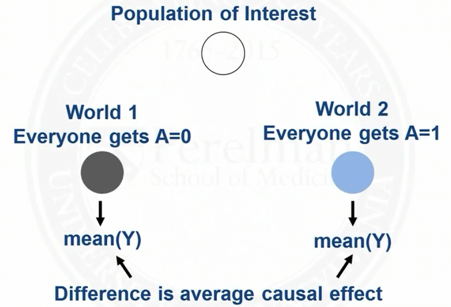
However, with certain assumptions, we can estimate population level (average) causal effects \(E(Y^1 - Y^0)\)
- Average value of \(Y\) if everyone was treated with \(A=1\) minus average value of \(Y\) if everyone was treated with \(A=0\)
- Headache example:
- Hopeless: What would have happened to me had I not taken ibuprofen? (Unit level causal effect)
- Hopeful: What would the rate of headache remission be if everyone took ibuprofen when they had a headache versus if no one did? (Population level causal effect)
Visualization of population average causal effect
Population average causal effect versus conditioning on treatment/control
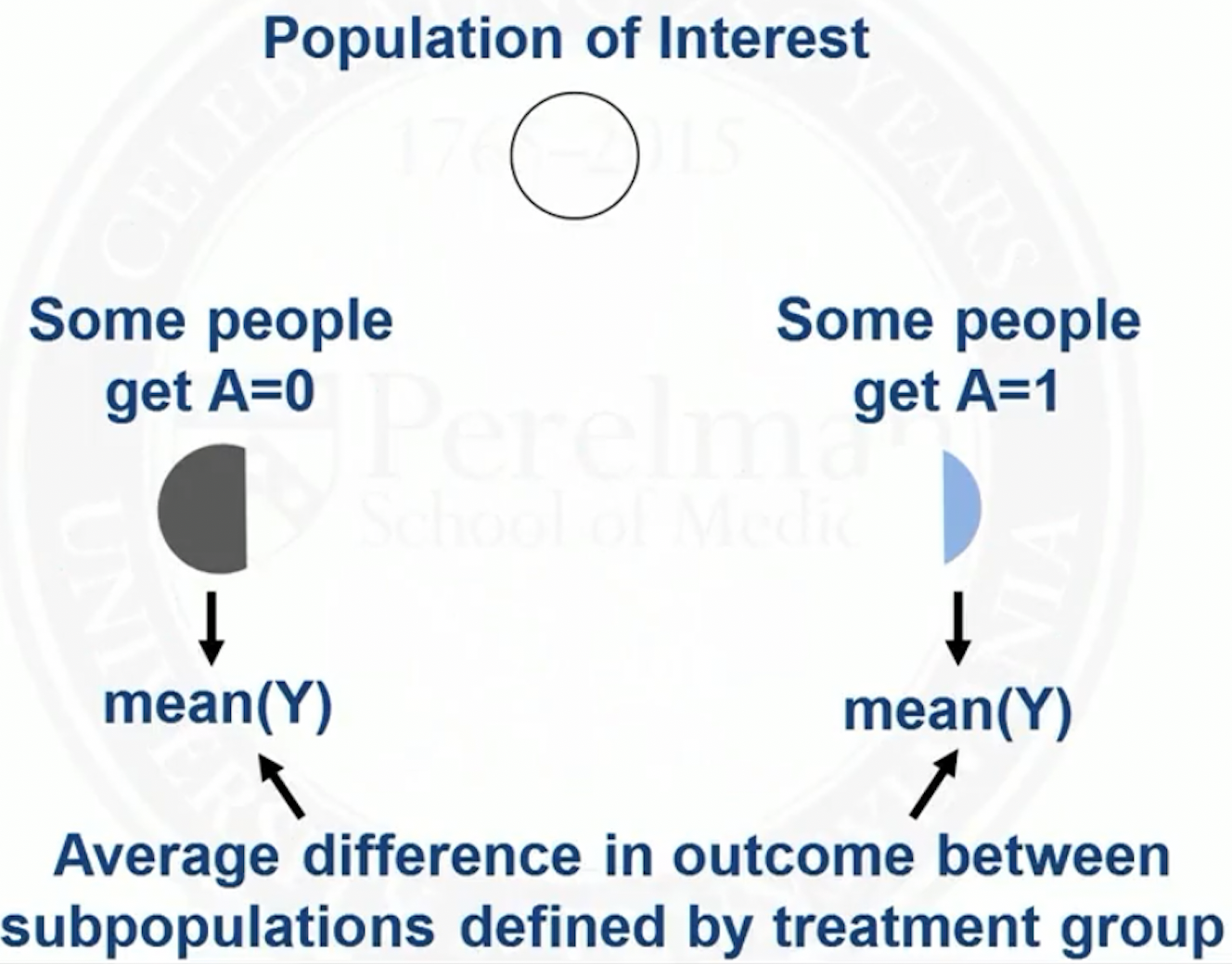
\[ E(Y^1 - Y^0) \neq E(Y\mid A=1) - E(Y\mid A=0) \]
In the left hand side, \(E(Y^1)\) is the mean of \(Y\) if the whole population was treated with \(A=1\)
In the right hand side, \(E(Y\mid A=1)\) is restricting to the subpopulation of people who actually had \(A=1\)
- This subpopulation may differ from the whole population in important ways
- For example, people at higher risk for flu are more likely to choose to get a flu shot
\(E(Y\mid A=1) - E(Y\mid A=0)\) is not a causal effect, because it is comparing two different populations of people
Visualization of real world
Other causal effects
\(E(Y^1 / Y^0)\): causal relative risk
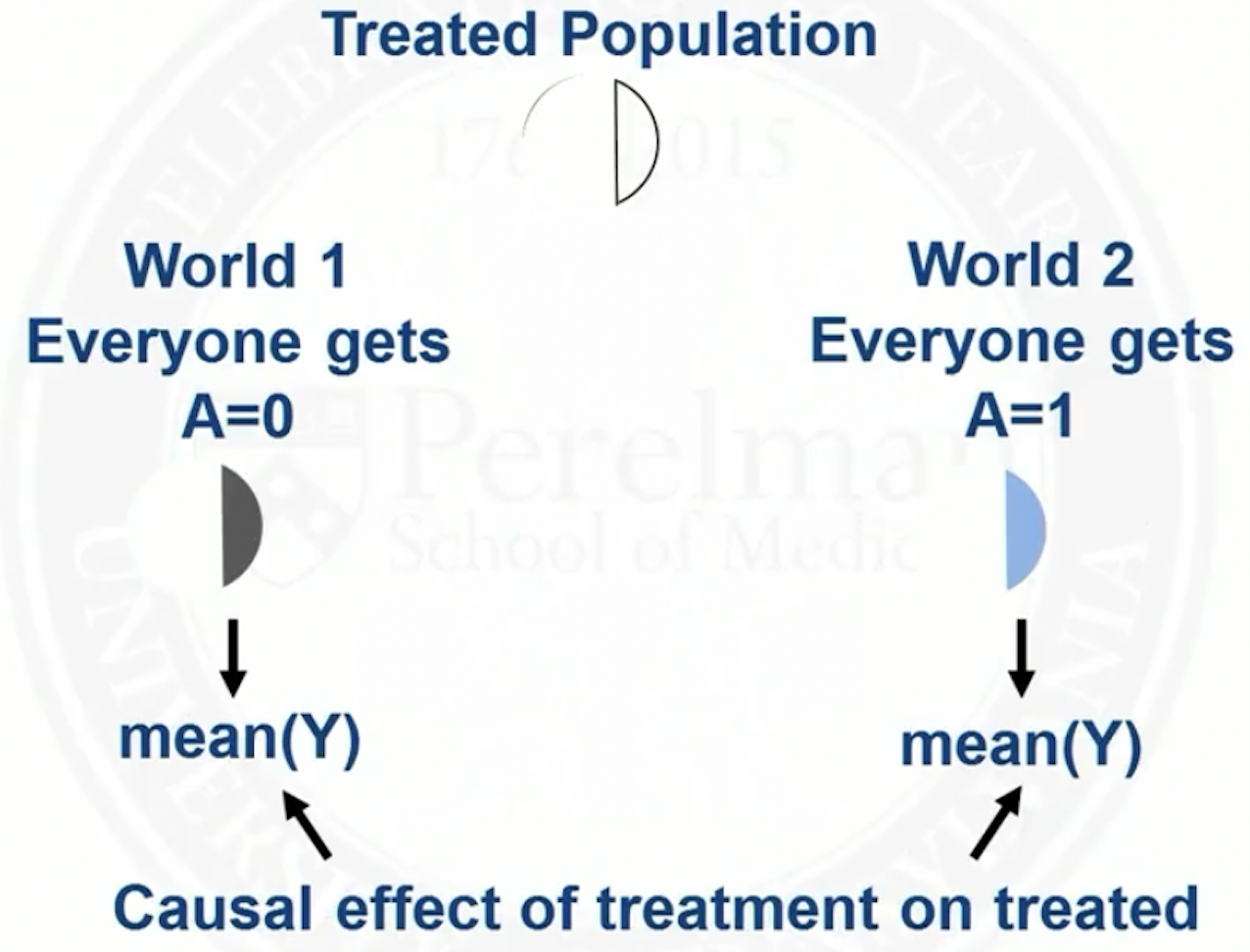
\(E(Y^1 - Y^0 \mid A=1)\): causal effect of treatment on the treated
\(E(Y^1 - Y^0 \mid V=v)\): average causal effect in the subpopulation with covariate \(V=v\)
Visualization of causal effect of treatment on the treated
Causal Assumptions
Most common causal assumptions
Stable Unit Treatment Value Assumption (SUTVA)
Consistency
Ignorability
Positivity
Stable Unit Treatment Value Assumption (SUTVA)
Stable Unit Treatment Value Assumption (SUTVA)
- SUTVA involves two assumptions
No interference
- Units do not interfere with each other
- Treatment assignement of one unit does not affect that outcome of another unit
- Spillover or contagion are also terms for interference
One version of treatment
- SUTVA allows us to write potential outcome for a person in terms of only that person’s treatments
Consistency
Consistency assumption
- Consistency assumption: the potential outcome under treatment \(A=a\), \(Y^a\), is equal to the observed outcome if the actual treatment received is \(A=a\)
\[ Y=Y^a \text{ if } A=a, \text{ for all } a \]
Ignorability
Ignorability assumption
Ignorability assumption: given pre-treatment covariates \(X\), treatment assignment is independent from the potential outcomes \[ Y^0, Y^1 \perp A \mid X \]
Among people with the same values of \(X\), we can think of treatment \(A\) as being randomly assigned
Example: \(Y^0\) and \(Y^1\) are not independent from \(A\) marginally, but within levels of \(X\), treatment might be randomly assigned
- \(X\): age; can take values ‘younger’ or ‘older’
- \(Y\): hip fracture
- Older people are more likely to get treatment \(A=1\)
- Older people are also more likely to have the outcome, regardless of treatment
Positivity
Positivity assumption
Positivity assumption: for every set of values of \(X\), treatment assignment was not deterministic \[ P(A=a \mid X=x) > 0, \text{ for all } a \text{ and } x \]
If for some values of \(X\), treatment was deterministic, then we would have no observed values of \(Y\) for one of the treatment groups for those values of \(X\)
Standardization and Stratification
Observed data and potential outcomes
- Under all above assumptions, the observed data average outcome \(E(Y\mid A=a, X=x)\) equals the potential outcomes \(E(Y^a \mid X=x)\)
\[\begin{align*} E(Y\mid A=a, X=x) &= E(Y^a\mid A=a, X=x) \text{ by consistency}\\ &= E(Y^a\mid X=x) \text{ by ignorability}\\ \end{align*}\]
- If we want a marginal causal effect, we can average over \(X\) \[ E(Y^a) = \sum_x E(Y \mid A=a, X=x) P(X=x) \]
Standardization
Standardization involves stratifying and then averaging
- First obtain the mean treatment effect within each stratum \(E(Y \mid A=a, X=x)\)
- Then pool across stratum, weighing by the probability (size) of each stratum \(P(X=x)\)
Standardization example: two diabetes treatments
Treatments: saxagliptin (new medicine) vs sitagliptin
Outcome: major adverse cardiac event (MACE)
Covariate: past use of oral antidiabetic (OAD) drug
Challenge
- Saxa users were more likely to have past use of OAD drug
- Patients with past use of OAD drugs are at higher risk of MACE
Stratify parents in two subpopulations by whether having prior OAD use
- Within levels of the prior OAD use variable, treatment can be thought of as randomized (ignorability)
Example continued: unstratified
| MACE=yes | MACE=no | Total | |
|---|---|---|---|
| Saxa=yes | 350 | 3650 | 4000 |
| Saxa=no | 500 | 6500 | 7000 |
| Total | 850 | 10150 | 11000 |
\[\begin{align*} &P(\text{MACE} \mid \text{Saxa}=\text{yes}) = 350/4000 = 0.088\\ &P(\text{MACE} \mid \text{Saxa}=\text{no}) = 500/7000 = 0.071 \end{align*}\]
Example continued: subpopulation without prior OAD use
| MACE=yes | MACE=no | Total | |
|---|---|---|---|
| Saxa=yes | 50 | 950 | 1000 |
| Saxa=no | 200 | 3800 | 4000 |
| Total | 250 | 4750 | 5000 |
\[\begin{align*} &P(\text{MACE} \mid \text{Saxa}=\text{yes}) = 50/1000 = 0.05\\ &P(\text{MACE} \mid \text{Saxa}=\text{no}) = 200/4000 = 0.05 \end{align*}\]
Example continued: subpopulation with prior OAD use
| MACE=yes | MACE=no | Total | |
|---|---|---|---|
| Saxa=yes | 300 | 2700 | 3000 |
| Saxa=no | 300 | 2700 | 3000 |
| Total | 600 | 5400 | 6000 |
\[\begin{align*} &P(\text{MACE} \mid \text{Saxa}=\text{yes}) = 300/3000 = 0.10\\ &P(\text{MACE} \mid \text{Saxa}=\text{no}) = 300/3000 = 0.10 \end{align*}\]
Example continued: mean potential outcome for Saxa
\[\begin{align*} & E(Y^{\text{saxa}})\\ = ~& E(Y\mid A=\text{saxa}, X = \text{prior OAD use yes}) P(\text{prior OAD use yes})\\ & + E(Y\mid A=\text{saxa}, X = \text{prior OAD use no}) P(\text{prior OAD use no})\\ = & (300/3000) (6000/11000) + (50/1000) (5000/11000) \\ = & 0.077 \end{align*}\]
Similarly, \(E(Y^{\text{sita}}) = 0.077\)
Hence, the treatment Saxa or not has no causal effects on the MACE outcome
Problems with standardization
There will be many \(X\) variables needed to achieve ignorability
Stratification would lead to many empy cells
Alternative to standardization: matching inverse probability of treatment weighting (IPTW), etc
References
Coursera class: “A Crash Course on Causality: Inferring Causal Effects from Observational Data”, by Jason A. Roy (University of Pennsylvania)