For the pdf slides, click here
Matching
Experiments vs observational studies
Randomized trials
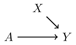
In experiments, treatment \(A\) is determined by a coin toss; so there are no arrows from \(X\) to \(A\), i.e., no backdoor paths
Covariate balance: distribution of pre-treatment variables \(X\) are the same in both treatment groups
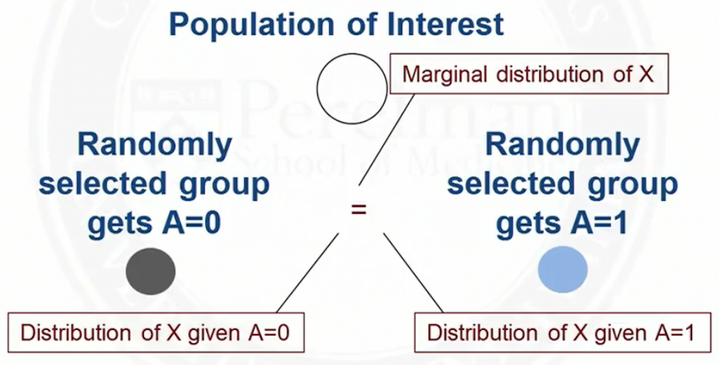
- Hence, if there is difference in the outcome, it is not because of \(X\)
Observational studies
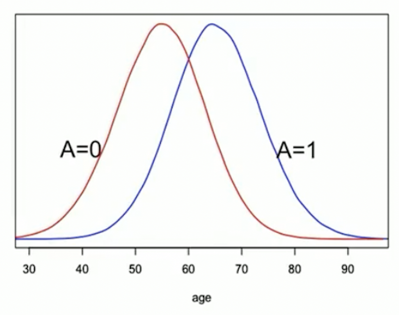
In observational studies, the distribution of \(X\) may differ between treatment groups
For example, older people may be more likely to get treatment \(A=1\):
Overview of matching
Matching
Matching: a method that attempts to make an observational study more like a randomized trial
Main idea of matching: match individuals in the treated group \((A=1)\) to individuals in the control group \((A=0)\) on the covariates \(X\)
- Usually, the sample size of the treated group is smaller than the control group, so after matching, we will use all cases in the treated group, but only a fraction of the cases in the control group
In the example where older people are more likely to get \(A=1\)
- At younger (older) ages, there are more people with \(A=0\) (\(A=1\))
In a randomized trial, for any particular age, there should be about the same number of treated and untreated people
This balance can be achieved by matching treated people to control people of the same age
Advantages of matching
Controlling for confounders is achieved at the design phase, i.e., without looking at the outcome
Matching will reveal lack of overlap in covariate distribution
- Positivity assumption will hold in the population that can be matched
We can treated a matched dataset as if from a randomized trial
Outcome analysis is simple
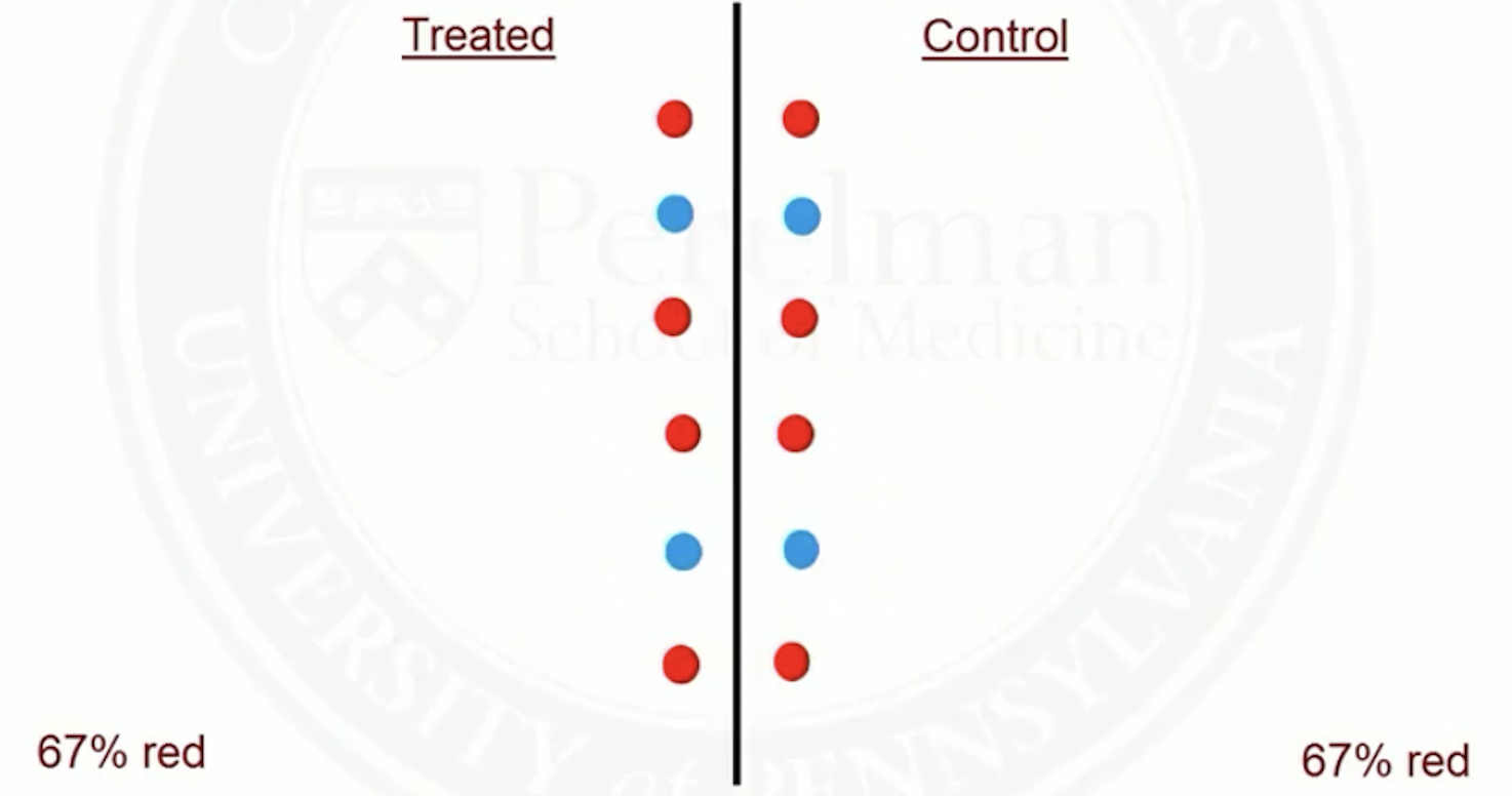
Match on a single covariate
Suppose red patients are more likely to be treated than blue ones
Before matching
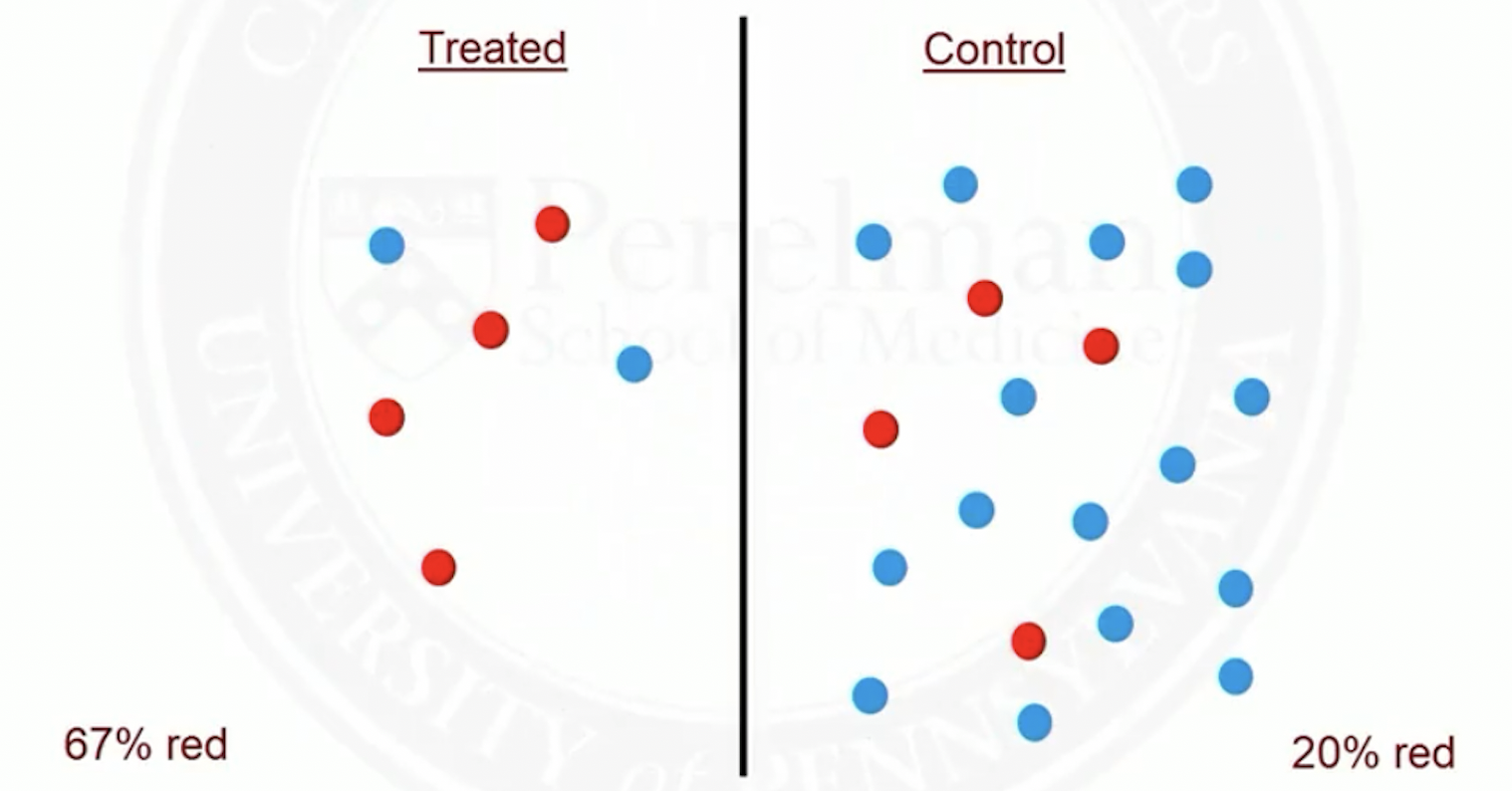
- After matching
Match on many covariates
We will not be able to exactly match on the full set of covariates
In randomized trials, treated and control subjects are not perfect matches either; the distribution of covariates is balanced between groups (stochastic balance)
Matching closely on covariates can achieve stochastic balance
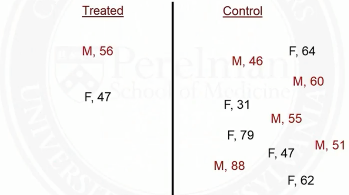
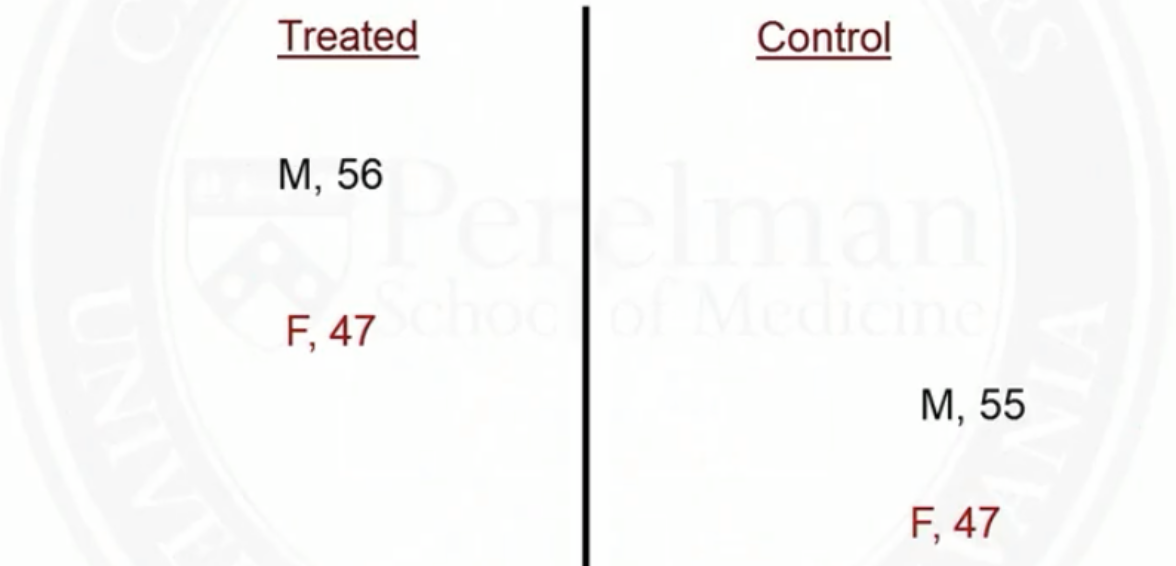
Example of matching on two covariates: sex and age
- Before matching
- After matching
Target population of matching: the treated
By matching, we are making the distribution of covariates in the control population look like that in the treated population
So we will analysis causal effect of treatment on the treated
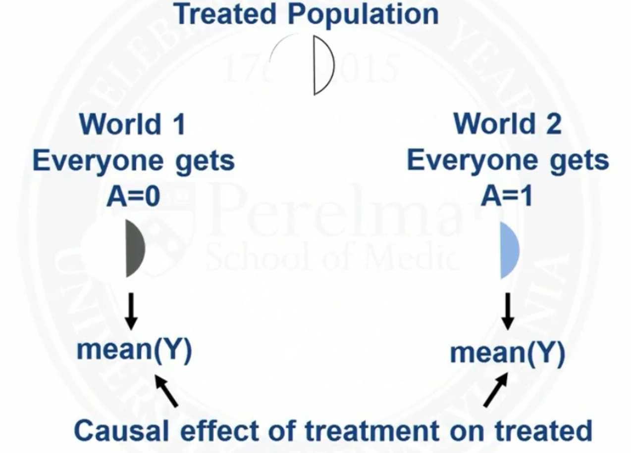
- There are matching methods that can be used to target a different population (beyond scope of this course)
Fine balance
Sometimes it is hard to find great matches, so we are willing to accept some non-ideal matches, if treated and control groups have the same distribution of covariates (fine balance)
For the matches below, average age and percent female are the same in both groups, although neither match is great
- Match 1: treated, male, age 40 and control, female, age 45
- Match 2: treated, female, age 45 and control, male, age 40
Number of matches
One to one (pair matching): match one control to every treated subject
Many to one: match \(K\) (a fixed number) controls to every treated subject; e.g., 5 to 1 matching
Variable: sometime match 1, sometimes more than 1 (if multiple good matches available), control to treated subjects
Metrics used in matching
Mahalanobis distance between two vectors: \[ D(\mathbf{X}_i, \mathbf{X}_j) = \sqrt{(\mathbf{X}_i - \mathbf{X}_j)^T \mathbf{S}^{-1}(\mathbf{X}_i - \mathbf{X}_j)}, \quad \mathbf{S} = cov(\mathbf{X}) \]
- We use covariance to scale so that the M distance is invariant of unit change
Robust Mahalanobis distance: robust to outliers
- Replace each covariate value with its rank
- Constant diagonal on covariance matrix
- Calculate the usual M distance on the ranks
Types of matching
- Greedy (nearest neighbor) matching
- Not ideal, but computationally fast
- Optimal matching
- Better, but computationally demanding
Nearest neighbor matching
Setup
We have selected a set of pre-treatment covariates \(X\) that satisfy the ignorability assumption
We have calculated a distance \(d_{i,j}\) between each treated subject \(i\) and each control subject \(j\)
We have more control subjects than the treated subjects
We will focus on pair matching (one-to-one)
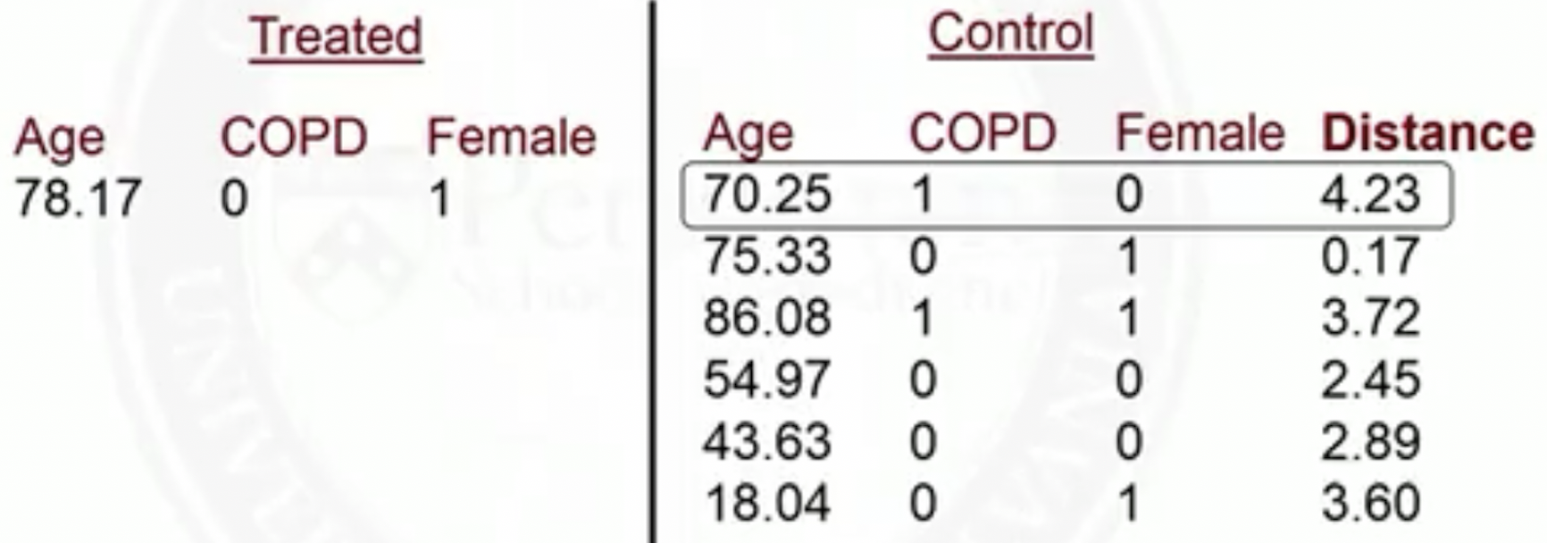
Nearest neighbor matching (greedy)
Randomly order list of treated subjects and control subjects
Start with the first treated subject, match to the control with the smallest distance
Remove the matched control from the list of available matches
Move on to the next treated subject. Repeat until all treated subjects are matched
Not invariant to order initial order of list
Not optimal: always taking the smallest distance match does not minimize total distance
R package: MatchIt, https://cran.r-project.org/web/packages/MatchIt/MatchIt.pdf
Many-to-one matching
For \(K\):1 matching: after everyone has 1 match, go through the list again and find 2nd matches. Repeat until \(K\) matches
Pair matching (one-to-one) vs many-to-one matching: a bias-variance tradeoff
Pair matching: closer matches, faster computing time
Many-to-one matching: larger sample size
Caliper
We may exclude a treated subject if there is no good matches for it
Caliper: maximum acceptable distance
- Only match a treated subject if the best match has distance less than the caliper
If no matches within caliper, it is a sign of violation of the positivity assumption. So we should exclude these subjects
Drawback: population harder to define
Optimal matching
Optimal matching
Optimal matching: minimized global distance measure, e.g., total distance
Computational feasibility of optimal matching: depends on the size of the problem
Number of treatment-control pairing: product of number of treatment and number of control
1 million treatment-control pairings is feasible on most computers (not quick, though)
1 billion pairings is not feasible
R packages: optmatch, rcbalance
Assessing matching balance
Assessing matching balance
- Check covariate balance: compute standardized difference to see if each covariate has similar means between treatment and control
\[
smd = \frac{\bar{X}_{\text{treatment}} - \bar{X}_{\text{control}}}{\sqrt{\frac{s^2_{\text{treatment}} + s^2_{\text{control}}}{2}}}
\]
- Does not depend on sample size
- Often, absolute value of smd is reported
- We calculate smd for each variable we match on
- This analysis does not involve the outcome variable
Rule of thumb:
- \(|smd| < 0.1\): adequate balance
- \(|smd| \in [0.1, 0.2]\): not too alarming
- \(|smd| > 0.2\): serious imbalance
Example: right heat characterization (RHC) data
- Table 1: compares pre-matching and post-matching balance
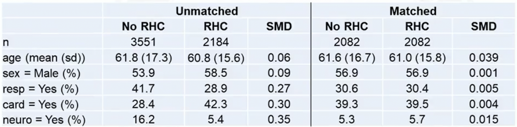
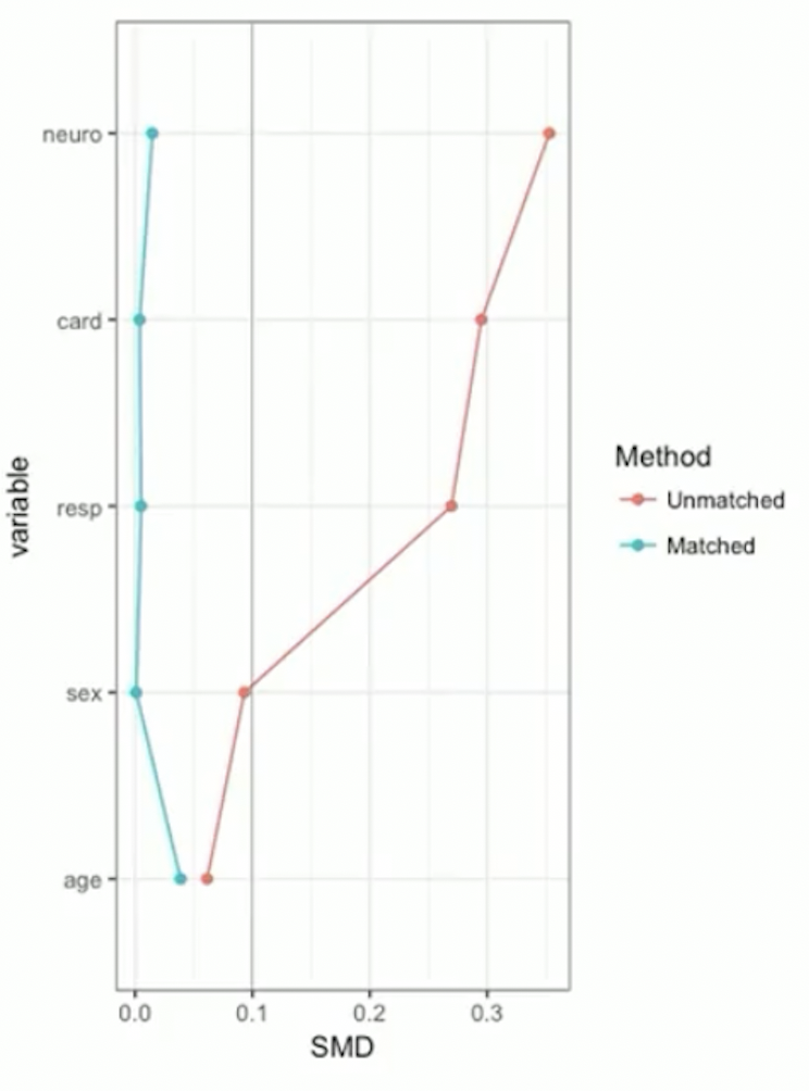
Example continued: RHC data
- SMD plot: visualizes Table 1
Analyze data after matching
After matching, proceed with outcome analysis
Test for a treatment effect
Estimate a treatment effect and confidence interval
Methods should take matching into account
Randomization test
Also known as permutation tests or exact tests
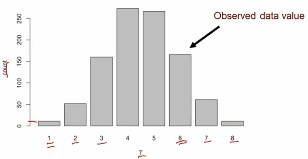
Main ideas of randomization test
Compute test statistic from observed data, assuming null hypothesis of no treatment effect is true
Randomly permute treatment assignment within pairs and recompute test statistic
Repeat many times and see how unusual observed statistic is
A binary outcome example
Test statistic: the total number of events in the treated group
- Test stat \(T=6\) in the observed data
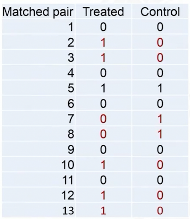
- In the observed data, discordant pairs (in red) are the only ones can change during treatment permutation
Permutation test for binary outcome: equivalent to a NcNemar test
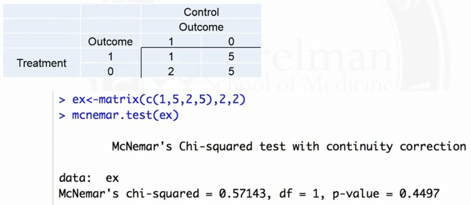
NcNemar test: whether row and column marginal frequencies are the same, for paired binary data
- Paired binary data, represented in a 2 by 2 contingency table
| Test 2 positive | Test 2 negative | Row total | |
|---|---|---|---|
| Test 1 positive | \(a\) | \(b\) | \(a+b\) |
| Test 1 negative | \(c\) | \(d\) | \(c+d\) |
| Column total | \(a+c\) | \(b+d\) | \(N\) |
Hypotheses: whether \(p_a + p_b = p_a + p_c\), or equivalently, \[ H_0: p_b = p_c, \quad H_1: p_b \neq p_c \]
Test statistic \[ \frac{(b-c)^2}{b+c} \stackrel{\text{under } H_0}{\sim} \chi^2_{df=1} \]
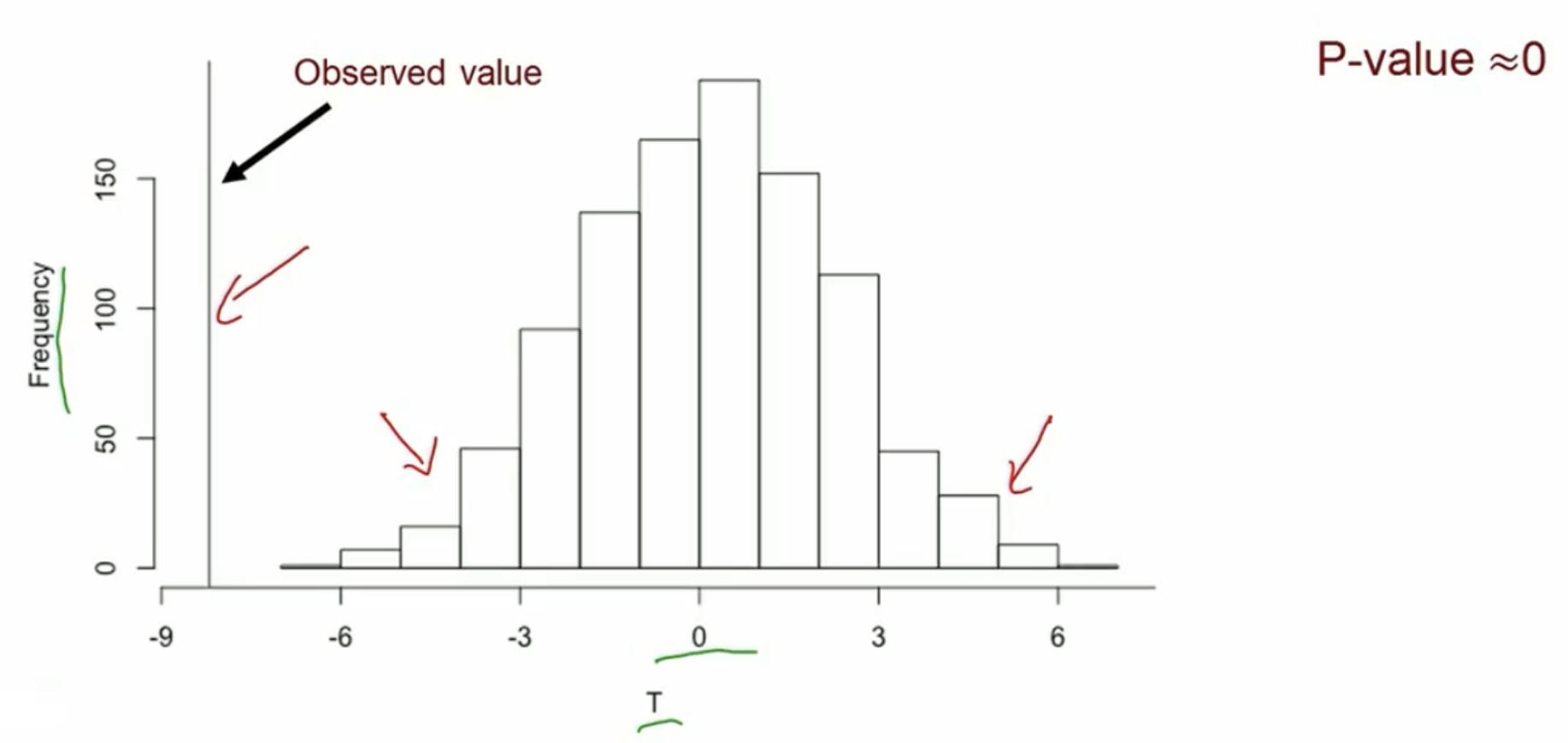
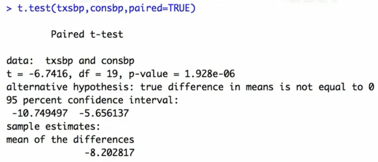
Permutation test for continuous outcome: equivalent to a paired t-test
- Test statistic: difference in sample means
Other outcome models
Conditional logistic regression
- Matched binary outcome data
Generalized estimating equations (GEE)
- Match ID variable used to specify clusters
- For binary outcomes, can estimate a causal risk difference, causal risk ratio, or causal odds ratio (depending on link function)
Propensity Score
Propensity score
Propensity score: probability of receiving treatment, given covariates \(X\) \[ \pi_i = P(A_i = 1 \mid X_i) \]
Propensity score is a balancing score \[ P(X = x \mid \pi(X) = p, A = 1) = P(X = x \mid \pi(X) = p, A = 0) \]
- Suppose two subjects have the same value of propensity score, but different covariate values \(X\)
- This means that both subjects’ \(X\) is just as likely to be found in the treatment group
- So if we restrict to a subpopulation of subjects who have the same value of the propensity score, there should be balance in the treatment vs control groups
We can match on propensity score to achieve balance
Logistic regression to estimate propensity score
In a randomized trial, the propensity score is known \[P(A=1\mid X) = P(A=0\mid X) = 0.5\]
In an observational study, we need to estimate the propensity score \(P(A=1\mid X)\)
- Fit a logistic regression: outcome \(A\), covariates \(X\)
- Get the predicted probability (fitted value) for each subject as the estimated propensity score
Propensity score matching
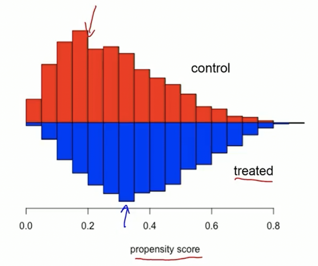
Before propensity score matching: check for overlap
Propensity score matching is simple; it’s matching on one variable
After the propensity is estimated, but before matching, it is useful to look for overlap
- This is to check positivity assumption
Example of good overlap
Trim tails if there is a lack of overlap
- Example of bad overlap
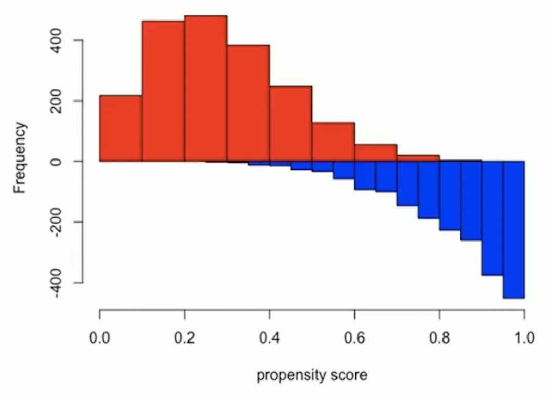
Trim tails: remove subjects who have extreme values of propensity score
- Remove control subjects whose propensity score is less than the minimum in the treatment group
- Remove treated subjects whose propensity score is greater than the maximum in the control group
Propensity score matching
Compute a distrance between the propensity score for each treated subject with every control
Use nearest neighbor or optimal matching
In practice, logit of the propensity score is often used, rather than the propensity score itself
A caliper can be used to avoid bad matches
- After matching: outcome analysis
- Randomization tests
- Conditional logistic regression, GEE, etc
References
Coursera class: “A Crash Course on Causality: Inferring Causal Effects from Observational Data”, by Jason A. Roy (University of Pennsylvania)