Week 3. Search
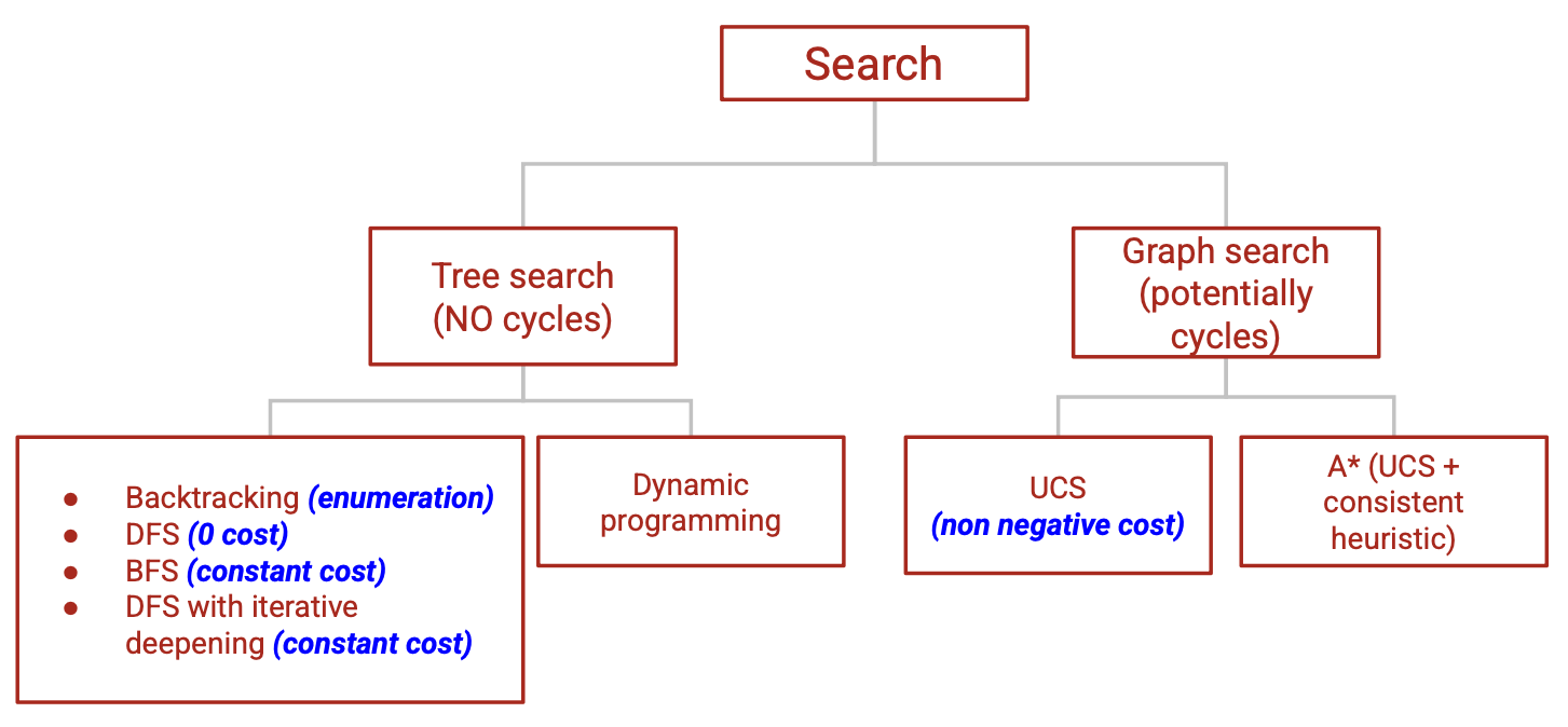
Figure source: Stanford CS221 spring 2025, Problem Workout 3 Slides
Note: DP is not necessarily a tree search algorithm. It’s a technique used to solve problems efficiently by breaking them down into smaller sub-problems. It can be applied to both tree search and graph search.
A good reference: state-based models cheetsheet
Tree Search
Model a search problem
Defining a search problem
- \(s_\text{start}\): stating state.
- Actions\((s)\): possible actions
- Cost\((s, a)\): action cost
- Succ\((s, a)\): the successor state
- IsEnd\((s)\): reached end state?
A search tree
- Node: a state
- Edge: an (action, cost) pair
- Root: starting state
- Leaf nodes: end states
Each root-to-leaf path represents a possible action sequence, and the sum of the costs of the edges is the cost of that path
Objective: find a minimal cost path to the end state
Coding a search problem: a class with the following methods:
stateState() -> StateisEnd(State) -> boolsuccAndCost(State) -> List[Tuple[str, State, float]]returns a list of(action, state, cost)tuples.
Tree search algorithms
- \(b\): actions per state, \(D\) maximum depth, \(d\) depth of the solution path
| Algorithm | Idea | Action costs | Space | Time |
|---|---|---|---|---|
| Backtracking search | Any cost | \(O(D)\) | \(O(b^D)\) | |
| Depth-first search | Backtracking + stop when find the first end state | All costs \(c\) = 0 | \(O(D)\) | \(O(b^D)\) |
| Breadth-first search | Explore in order of increasing depth | Constant cost \(c\geq 0\) | \(O(b^d)\) | \(O(b^d)\) |
| DFS with iterative deepening | Call DFS for maximum depths 1, 2, \(\ldots\) | Constant cost \(c\geq 0\) | \(O(d)\) | \(O(b^d)\) |
- Always exponential time
- Avoid exponential spaces with DFS-ID
Dynamic Programming
Dynamic programming (DP)
- A backtracking search algorithm with memorization (i.e. partial results are saved)
- May avoid the exponential running time of tree search
- Assumption: acyclic graph, so there is always a clear order in which to compute all the future (or past) costs.
For any given state \(s\), the DP future cost is \[ \text{FutureCost}(s) = \begin{cases} 0 & \text{ if IsEnd}(s)\\ \min_{a \in \text{Actions}(s)} \left[\text{Cost}(s, a) + \text{FutureCost}(\text{Succ}(s, a)) \right] & \text{ otherwise} \end{cases} \]
Note that for DP, we can analogously define \(\text{PastCost}(s)\).
A state is a summary of all the past actions sufficient to choose future actions optimally.
Graph Search
- \(N\) total states, \(n\) of which are closer than end state
| Algorithm | Cycles? | Idea | Action costs | Time/space |
|---|---|---|---|---|
| Dynamic programming | No | Save partial results | Any | \(O(N)\) |
| Uniform cost search | Yes | Enumerates states in order of increasing past cost | \(\text{Cost}(s, a) \geq 0\) | \(O(n\log n)\) |
- Exponential savings compared with tree search!
- Graph search: can have cycles
Uniform cost search (UCS)
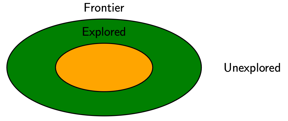
Figure source: Stanford CS221 spring 2025, lecture slides week 3
Types of states
- Explored: optimal path found; will not update cost to these states in the future
- Frontier: states we’ve seen, but still can update the cost of how to get there cheaper (i.e., priority queue)
- Unexplored: states we haven’t seen
Uniform cost search (UCS) algorithm
- Add \(s_{\text{start}}\) to frontier
- Repeat until fronteir is empty:
- Remove \(s\) with smallest priority (minimum cost to \(s\) among visited paths) \(p\) from frontier
- If \(\text{IsEnd}(s)\): return solution
- Add \(s\) to explored
- For each action \(a \in \text{Actions(s)}\):
- Get successor \(s' \leftarrow \text{Succ}(s, a)\)
- If \(s'\) is already in explored: continue
- Update frontier with \(s'\) and priority with \(p + \text{Cost}(s, a)\) (if it’s cheaper)
Properties of UCS
Correctness: When a state \(s\) is popped from the frontier and moved to explored, its priority is PastCost\((s)\), the minimum cost to \(s\).
USC potentially explores fewer states, but requires move overhead to maintain the priority queue
A*
A* algorithm: Run UCS with modified edge costs \[ \text{Cost}'(s, a) = \text{Cost}(s, a) + h(\text{Succ}(s, a)) - h(s) \]
- USC: explore states in order of PastCost\((s)\)
- A*: explore states in order of PastCost\((s) + h(s)\)
- \(h(s)\) is a heuristic that estimates FutureCost\((s)\)
Heuristic \(h\)
Consistency:
- Triangle inequality: \(\text{Cost}'(s, a) = \text{Cost}(s, a) + h(\text{Succ}(s, a)) - h(s) \geq 0\), and
- \(h(s_\text{end}) = 0\)
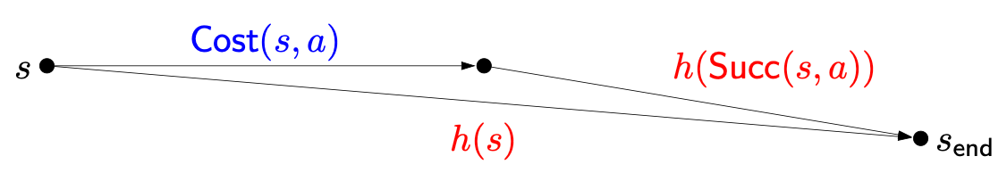
Figure source: Stanford CS221 spring 2025, lecture slides week 3
Admissibility: \[h(s) \leq \text{FutureCost}(s)\]
If \(h(s)\) is consistent, then it is admissible.
A* properties
- Correctness: if \(h\) is consistent, then A* returns the minimum cost path
- Efficiency: A* explores all states \(s\) satisfying
\[\text{PastCost}(s) \leq \text{PastCost}(s_\text{end}) - h(s)\]
- If \(h(s)=0\), then A* is the same as UCS
- If \(h(s)=\text{FutureCost}(s)\), then A* only explores nodes on a minimum cost path
- Usually somewhere in between
Create \(h(s)\) via relaxation
- Remove constraints
- Reduce edge costs (from \(\infty\) to some finite cost)
Week 4. Markov Decision Processes
- Uncertainty in the search process
- Performing action \(a\) from a state \(s\) can lead to several states \(s'_1, s'_2, \ldots\) in a probabilistic manner.
- The probability and reward of each \((s, a, s')\) pair may be known or unknown.
- If known: policy evaluation, value iteration
- If unknown: reinforcement learning
Markov Decision Processes (offline)
Model an MDP
- Markove decision process definition:
- States: the set of states
- \(s_\text{start}\): stating state.
- Actions\((s)\): possible actions
- \(T(s, a, s')\): transition probability of \(s'\) if take action \(a\) in state \(s\)
- Reward\((s, a, s')\): reward for the transition \((s, a, s')\)
- IsEnd\((s)\): reached end state?
- \(\gamma \in (0, 1]\): discount factor
- A policy \(\pi\): a mapping from each state \(s \in \text{States}\) to an action \(a \in \text{Actions}(s)\)
Policy Evaluation (on-policy)
Utility of a policy is the discounted sum of the rewards on the path
- Since the policy yields a random path, its utility is a random variable
For a policy, its path is \(s_0, a_1 r_1 s_1, a_2r_2s_2, \ldots\) (action, reward, new state) tuple, then the utility with discount \(\gamma\) is \[ u_1 = r_1 + \gamma r_2 + \gamma^2 r_3 + \ldots \]
\(V_\pi(s)\): the expected utility (called value) of a policy \(\pi\) from state \(s\)
\(Q_\pi(s, a)\): Q-value, the expected utility of taking action \(a\) from state \(s\), and then following policy \(\pi\)
Connections between \(V_\pi(s)\) and \(Q_\pi(s, a)\):
\[ V_\pi(s) = \begin{cases} 0 & \text{ if IsEnd}(s)\\ Q_\pi(s, \pi(s)) & \text{ otherwise} \end{cases} \]
\[ Q_\pi(s, a) = \sum_{s'} T(s, a, s')\left[\text{Reward}(s, a, s') + \gamma V_\pi(s')\right] \]
Iterative algorithm for policy evaluation
- Initialize \(V_\pi^{(0)}(s) = 0\) for all \(s\)
- For iteration \(t = 1, \ldots, t_\text{PE}\):
- For each state \(s\), \[V_\pi^{(t)}(s) = \sum_{s'} T\left(s, \pi(s), s'\right)\left[\text{Reward}\left(s, \pi(s), s'\right) + \gamma V_\pi^{(t-1)}(s')\right]\]
Choice of \(t_\text{PE}\): stop when values don’t change much \[ \max_{s} \left|V_\pi^{(t)}(s) - V_\pi^{(t-1)}(s)\right| \leq \epsilon \]
MDP time complexity is \(O(t_\text{PE} S S')\), where \(S\) is the number of states and \(S'\) is the number of \(s'\) with \(T(s, a, s') \geq 0\)
Value Iteration (off-policy)
Optimal value \(V_\text{opt}(s)\): maximum value attained by any policy
Optimal Q-value \(Q_\text{opt}(s, a)\)
\[ Q_\text{opt}(s, a) = \sum_{s'} T(s, a, s') \left[\text{Reward}(s, a, s') + \gamma V_{opt}(s') \right] \]
\[ V_\text{opt}(s) = \begin{cases} 0 & \text{ if IsEnd}(s)\\ \max_{a\in \text{Actions}(s)} Q_\text{opt}(s, a) & \text{ otherwise} \end{cases} \]
- Value iteration algorithm:
- Initialize \(V_\text{opt}^{(0)}(s) = 0\) for all \(s\)
- For iteration \(t = 1, \ldots, t_\text{VI}\):
- For each state \(s\), \[V_\text{opt}^{(t)}(s) = \max_{a\in \text{Actions}(s)} \sum_{s'} T\left(s, a, s'\right)\left[\text{Reward}\left(s, a, s'\right) + \gamma V_\text{opt}^{(t-1)}(s)\right]\]
- VI time complexity is \(O(t_\text{VI} S A S')\), where \(S\) is the number of states, \(A\) is the number of actions, and \(S'\) is the number of \(s'\) with \(T(s, a, s') \geq 0\)
Reinforcement Learning (online)
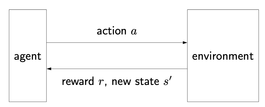
Figure source: Stanford CS221 spring 2025, lecture slides week 4
- Summary of reinforcement learning algorithms
| Algorithm | Estimating | Based on |
|---|---|---|
| Model-based Monte Carlo | \(\hat{T}, \hat{R}\) | \(s_0, a_1, r_1, s_1, \ldots\) |
| Model-free Monte Carlo | \(\hat{Q}_\pi\) | \(u\) |
| SARSA | \(\hat{Q}_\pi\) | \(r + \hat{Q}_\pi\) |
| Q-learning | \(\hat{Q}_\text{opt}\) | \(r + \hat{Q}_\text{opt}\) |
Model-based methods (off-policy)
\[ \hat{Q}_\text{opt}(s, a) = \sum_{s'} \hat{T}(s, a, s') \left[\widehat{\text{Reward}}(s, a, s') + \gamma \hat{V}_{opt}(s') \right] \]
- Based on data \(s_0; a_1, r_1, s_1; a_2, r_2, s_2; \ldots ; a_n, r_n, s_n\), estimate the transition probabilities and rewards of the MDP
\[\begin{align*} \hat{T}(s, a, s') & = \frac{\# \text{times } (s, a, s') \text{ occurs}} {\# \text{times } (s, a) \text{ occurs}} \\ \widehat{\text{Reward}}(s, a, s') & = r \text{ in } (s, a, r, s') \end{align*}\]
- If \(\pi\) is a non-deterministic policy which allows us to explore each (state, action) pair infinitely often, then the estimates of the transitions and rewards will converge.
- Thus, the estimates \(\hat{T}\) and \(\widehat{\text{Reward}}\) are not necessarily policy dependent. So model-based methods are off-policy estimations.
Model-free Monte Carlo (on-policy)
The main idea is to estimate the Q-values directly
Original formula \[ \hat{Q}_\pi (s, a) = \text{average of } u_t \text{ where } s_{t-1} = s, a_t = a \]
Equivalent formulation: for each \((s, a, u)\), let \[\begin{align*} \eta & = \frac{1}{1 + \#\text{updates to }(s, a)}\\ \hat{Q}_\pi(s, a) & \leftarrow (1-\eta) \underbrace{\hat{Q}_\pi (s, a)}_{\text{prediction}} + \eta \underbrace{u}_{\text{data}}\\ & = \hat{Q}_\pi (s, a) - \eta\left(\hat{Q}_\pi (s, a) - u\right) \end{align*}\]
- Implied objective: least squares \[\left(\hat{Q}_\pi (s, a) - u \right)^2\]
SARSA (on-policy)
- SARSA algorithm
On each \((s, a, r, s', a')\): \[ \hat{Q}_\pi(s, a) \leftarrow (1-\eta) \hat{Q}_\pi(s, a) + \eta \left[\underbrace{r}_{\text{data}} + \gamma \underbrace{\hat{Q}_\pi(s', a')}_{\text{estimate}}\right] \]
- SARSA uses estimates \(\hat{Q}_\pi(s', a')\) instead of just raw data \(u\)
| Model-free Monte Carlo | SARSA |
|---|---|
| \(u\) | \(r + \hat{Q}_\pi(s', a')\) |
| based on one path | based on estimate |
| unbiased | biased |
| large variance | small variance |
| wait until end of update | can update immediately |
Q-learning (off-policy)
On each \((s, a, r, s')\): \[\begin{align*} \hat{Q}_\text{opt}(s, a) & \leftarrow (1-\eta) \underbrace{\hat{Q}_\text{opt}(s, a)}_{\text{prediction}} + \eta \underbrace{\left[r + \gamma \hat{V}_\text{opt}(s')\right]}_{\text{target}}\\ \hat{V}_\text{opt}(s') &= \max_{a' \in \text{Actions}(s')} \hat{Q}_\text{opt}(s', a') \end{align*}\]
Epsilon-greedy
Reinforcement learning algorithm template
- For \(t = 1, 2, 3, \ldots\)
- Choose action \(a_t = \pi_\text{act}(s_{t-1})\)
- Receive reward \(r_t\) and observe new state \(s_t\)
- Update parameters
- For \(t = 1, 2, 3, \ldots\)
What exploration policy \(\pi_\text{act}\) to use? Need to balance exploration and exploitation.
Epsilon-greedy policy \[ \pi_\text{act}(s) = \begin{cases} \arg\max_{a \in \text{Actions}(s)} \hat{Q}_\text{opt}(s, a) & \text{ probability } 1- \epsilon\\ \text{random from Actions}(s) & \text{ probability } \epsilon \end{cases} \]
Function appxomation
- Large state spaces is hard to explore.For better generalization to handle unseen states/actions, we can use function approximation, to define
- features \(\phi(s, a)\), and
- weights \(\mathbf{w}\), such that \[\hat{Q}_\text{opt}(s, a; \mathbf{w}) = \mathbf{w} \cdot \phi(s, a)\]
- Q-learning with function approximation: on each \((s, a, r, s')\),
\[ \mathbf{w} \leftarrow \mathbf{w} - \eta\left[ \underbrace{\hat{Q}_\text{opt}(s, a; \mathbf{w})}_{\text{prediction}} - \underbrace{\left(r + \gamma \hat{V}_\text{opt}(s') \right)}_{\text{target}} \right] \phi(s, a) \]
Week 5. Games
Modeling Games
- A simple example game
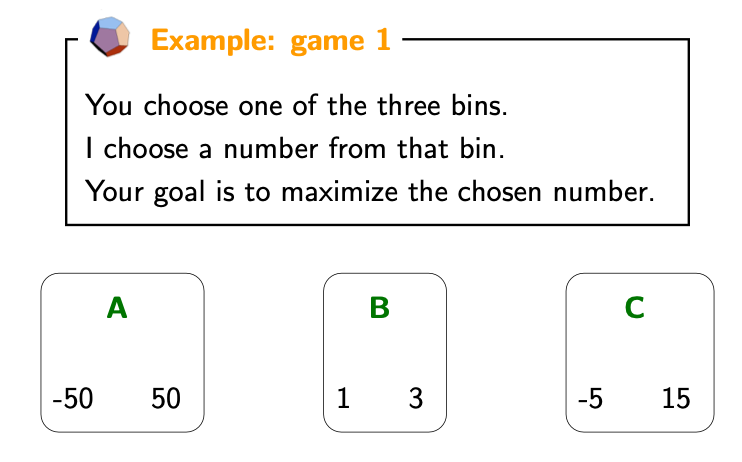
Figure source: Stanford CS221 spring 2025, lecture slides week 5
- Game tree
- Each node is a decision point for a player
- Each root-to-leaf path is a possible outcome of the game
- Nodes to indicate certain policy: use \(\bigtriangleup\) for maximum node (agent maximize his utility) and \(\bigtriangledown\) for minimum node (opponent minimizes agent’s utility)
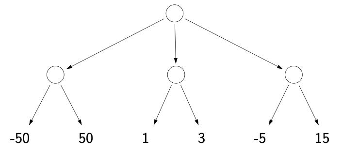
Figure source: Stanford CS221 spring 2025, lecture slides week 5
Two-player zero-sum game:
- \(s_\text{start}\)
- Actions\((s)\)
- Succ\((s, a)\)
- IsEnd\((s)\)
- Utility\((s)\): agent’s utility for end state \(s\)
- Player\((s) \in \text{Players}\): player who controls state s
- Players \(= \{\text{agent}, \text{opp} \}\)
- Zero-sum: utility of the agent is negative the utility of the opponent
Property of games
- All the utility is at the end state
- For a game about win/lose at the end (e.g., chess), Utility\((s)\) is \(\infty\) (if agent wins), \(-\infty\) (if opponent wins), or \(0\) (if draw).
- Different players in control at different state
- All the utility is at the end state
Policies (for player \(p\) in state \(s\))
- Deterministic policy: \(\pi_p(s) \in \text{Actions}(s)\)
- Stochastic policy: \(\pi_p(s, a) \in [0, 1]\), a probability
Game Algorithms
Game evaluation
- Use recurrence for policy evaluation to estimate value of the game (expected utility):
\[ V_\text{eval}(s) = \begin{cases} \text{Utility}(s) & \text{ IsEnd}(s)\\ \sum_{a\in\text{Actions}(s)} \pi_\text{agent}(s, a) V_\text{eval}(\text{Succ}(s, a)) & \text{ Player}(s) = \text{agent}\\ \sum_{a\in\text{Actions}(s)} \pi_\text{opp}(s, a) V_\text{eval}(\text{Succ}(s, a)) & \text{ Player}(s) = \text{opp}\\ \end{cases} \]
Expectimax
- Expectimax: given opponent’s policy, find the best policy for the agent
\[ V_\text{exptmax}(s) = \begin{cases} \text{Utility}(s) & \text{ IsEnd}(s)\\ \max_{a\in\text{Actions}(s)} V_\text{exptmax}(\text{Succ}(s, a)) & \text{ Player}(s) = \text{agent}\\ \sum_{a\in\text{Actions}(s)} \pi_\text{opp}(s, a) V_\text{exptmax}(\text{Succ}(s, a)) & \text{ Player}(s) = \text{opp}\\ \end{cases} \]
Minimax
- Minimax assumes the worst case for the opponent’s policy
\[ V_\text{minmax}(s) = \begin{cases} \text{Utility}(s) & \text{ IsEnd}(s)\\ \max_{a\in\text{Actions}(s)} V_\text{minmax}(\text{Succ}(s, a)) & \text{ Player}(s) = \text{agent}\\ \min_{a\in\text{Actions}(s)} V_\text{minmax}(\text{Succ}(s, a)) & \text{ Player}(s) = \text{opp}\\ \end{cases} \]
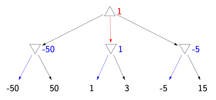
Figure source: Stanford CS221 spring 2025, lecture slides week 5
Minimax properties
- Best against minimax opponent \[ V(\pi_\max, \pi_\min) \geq V(\pi_\text{agent}, \pi_\min) \text{ for all } \pi_\text{agent} \]
- Lower bound against any opponent \[ V(\pi_\max, \pi_\min) \leq V(\pi_\max, \pi_\text{opp}) \text{ for all } \pi_\text{opp} \]
- Not optimal if opponent is known! Here, \(\pi_7\) stands for an arbitrary known policy, for example, random choice with equal probabilities. \[ V(\pi_\max, \pi_7) \geq V(\pi_{\text{exptmax}(7)}, \pi_7) \text{ for opponent } \pi_7 \]
Relationship between game values
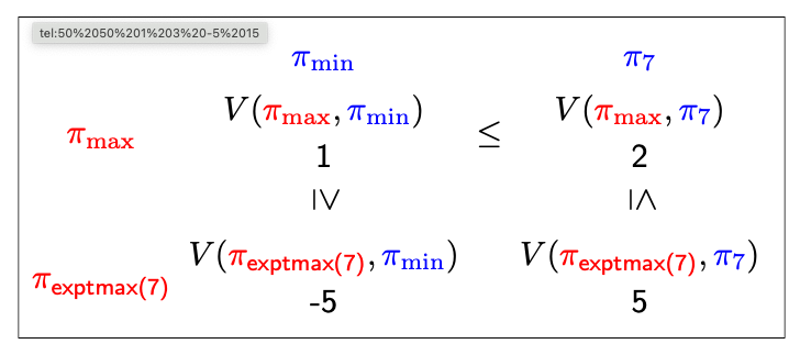
Figure source: Stanford CS221 spring 2025, lecture slides week 5
Expectiminimax
- Modify the game to introduce randomness
Figure source: Stanford CS221 spring 2025, lecture slides week 5
- This is equivalent to having a third player, the coin \[ V_\text{exptminmax}(s) = \begin{cases} \text{Utility}(s) & \text{ IsEnd}(s)\\ \max_{a\in\text{Actions}(s)} V_\text{exptminmax}(\text{Succ}(s, a)) & \text{ Player}(s) = \text{agent}\\ \min_{a\in\text{Actions}(s)} V_\text{exptminmax}(\text{Succ}(s, a)) & \text{ Player}(s) = \text{opp}\\ \sum_{a\in\text{Actions}(s)} \pi_\text{coin}(s, a) V_\text{exptminmax}(\text{Succ}(s, a)) & \text{ Player}(s) = \text{coin}\\ \end{cases} \]
Evaluation functions
Computation complexity: with branching factor \(b\) and depth \(d\) (number of turns \(2d\) because of two players), since this is a tree search, we have
- \(O(d)\) space
- \(O(b^{2d})\) time
Limited depth tree search: stop at maximum depth \(d_\max\) \[ V_\text{minmax}(s, d) = \begin{cases} \text{Utility}(s) & \text{ IsEnd}(s)\\ \text{Eval}(s) & d=0\\ \max_{a\in\text{Actions}(s)} V_\text{minmax}(\text{Succ}(s, a), d) & \text{ Player}(s) = \text{agent}\\ \min_{a\in\text{Actions}(s)} V_\text{minmax}(\text{Succ}(s, a), d-1) & \text{ Player}(s) = \text{opp}\\ \end{cases} \]
- Use: at state \(s\), call \(V_\text{minmax}(s, d_\max)\)
An evaluation function Eval\((s)\) is a possibly very weak estimate of the value \(V_\text{minmax}(s)\), using domain knowledge
- This is similar to FutureCost\((s)\) in the A* search problems. But unlike A*, there are no guarantees on the error for approximation.
Alpha-Beta pruning
Branch and bound
- Maintain lower and upper bounds on values.
- If intervals don’t overlap, then we can choose optimally without future work
Alpha-beta prining for minimax:
- \(a_s\): lower bound on value of max node \(s\)
- \(b_s\): upper bound on value of min node \(s\)
- Store \(\alpha_s = \max_{s'\leq s} a_{s'}\) and \(\beta_s = \min_{s'\leq s} b_{s'}\)
- Prune a node if its interval doesn’t have non-trivial overlap with every ancestor
Pruning depends on the order
- Worse ordering: \(O(b^{2\cdot d})\) time
- Best ordering: \(O(b^{2\cdot 0.5 d})\) time
- Random ordering: \(O(b^{2\cdot 0.75 d})\) time, when \(b=2\)
- In practice, we can order based on the evaluation function Eval\((s)\):
- Max nodes: order successors by decreasing Eval\((s)\)
- Min nodes: order successors by increasing Eval\((s)\)
More Topics
TD learning (on-policy)
General learning framework
- Objective function \[ \frac{1}{2}\left(\text{prediction}(\mathbf{w}) - \text{target} \right)^2 \]
- Update \[ \mathbf{w} \leftarrow \mathbf{w} - \eta \left(\text{prediction}(\mathbf{w}) - \text{target} \right) \nabla_\mathbf{w} \text{prediction}(\mathbf{w}) \]
Temporal difference (TD) learning: on each \((s, a, r, s')\),
\[ \mathbf{w} \leftarrow \mathbf{w} - \eta \left[V(s; \mathbf{w}) - \left(r + \gamma V(s'; \mathbf{w})\right) \right] \nabla_\mathbf{w} V(s; \mathbf{w}) \]
- For linear function \[V(s; \mathbf{w}) = \mathbf{w} \cdot \phi(s)\]
Simultaneous games
Payoff matrix: for two players, \(V(a, b)\) is A’s utility if A chooses action \(a\) and B chooses action \(b\)
Strategies (policies)
- Pure strategy: a single action
- Mixed strategy: a probability distribution of actions
Game evaluation: the value of the game if player A follows \(\pi_A\) and player B follows \(\pi_B\) is \[ V(\pi_A, \pi_B) = \sum_{a, b} \pi_A(a) \pi_B(b) V(a, b) \]
For pure strategies, going second is no worse \[\max_a \min_b V(a, b) \leq \min_b \max_a V(a, b)\]
Mixed strategy: second play can play pure strategy: for any fixed mixed strategy \(\pi_A\), \(\min_{\pi_B} V(\pi_A, \pi_B)\) can be obtained by a pure strategy
Minimax theorem: for every simultaneous two-player zero-sum game with a finite number of actions \[ \max_{\pi_A} \min_{\pi_B} V(\pi_A, \pi_B) = \min_{\pi_B}\max_{\pi_A} V(\pi_A, \pi_B) \]
- Revealing your optimal mixed strategy doesn’t hurt you.