For the pdf slides, click here
Concepts of MCAR, MAR, MNAR
Concepts of MCAR, MAR, MNAR
- Missing completely at random (MCAR): the probability of being missing is the same for all cases
- Cause of missing is unrelated to the data
- Missing at random (MAR): the probability of being missing only depends on the observed data
- Cause of missing is unrelated to the missing values
- Missing not at random (MNAR): probability of being missing depends on the missing values themselves
Ad-hoc Solutions
Listwise deletion and pairwise deletion
- Listwise deletion (also called complete-case analysis): delete rows which contain one or more missing values
- If data is MCAR, listwise deletion produces unbiased estimates of means, variances, and regression weights (if need to train a predictive model)
- If data is not MCAR, listwise deletion can severely bias the above estimates.
- Pairwise deletion (also called available-case analysis)
- Mean and variance of variable \(X\) are based on all cases with observed data on \(X\)
- Covariance and correlation of \(X\) and \(Y\) is based on all data which both \(X\) and \(Y\) have non-missing values
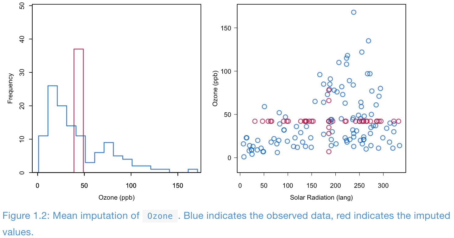
Mean imputation
- Compared with the observed data, in the imputed data (observed + imputed values)
- Standard deviations decrease
- Correlation decreases
- Means can be biased if the data is not MCAR.
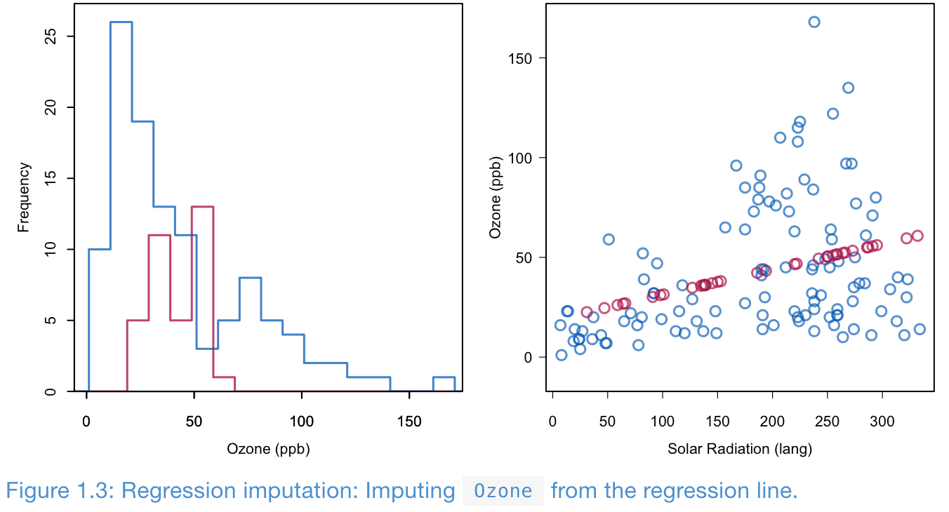
Regression imputation
- Build a regression model from the observed data
- Impute the missing values in the response variable with the predicted values from the fitted regression
- The impute values are the most likely values under the model
- However, it decreases the variance of the target variable
- And it increases the correlations between the target and covariates
- Regression imputation, and its modern incarnations in machine learning is probably the most dangerous of all ad-hoc methods
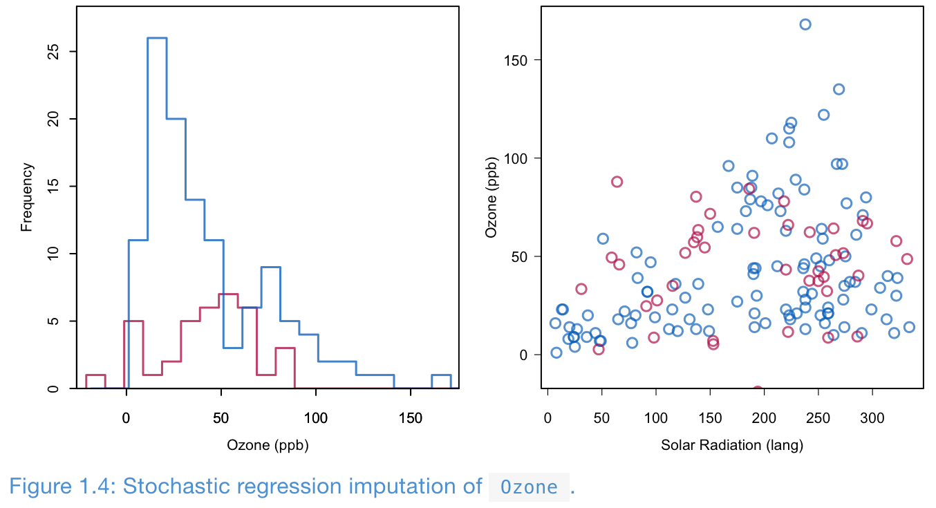
Stochastic regression imputation
- Build a regression model from the observed data
- Impute a missing value in the response variable with the predicted value plus a random draw from the residual
- Preserves variance and correlation.
- Imputed values can exceed the range (e.g., a negative Ozone level). A more suitable model may resolve this.
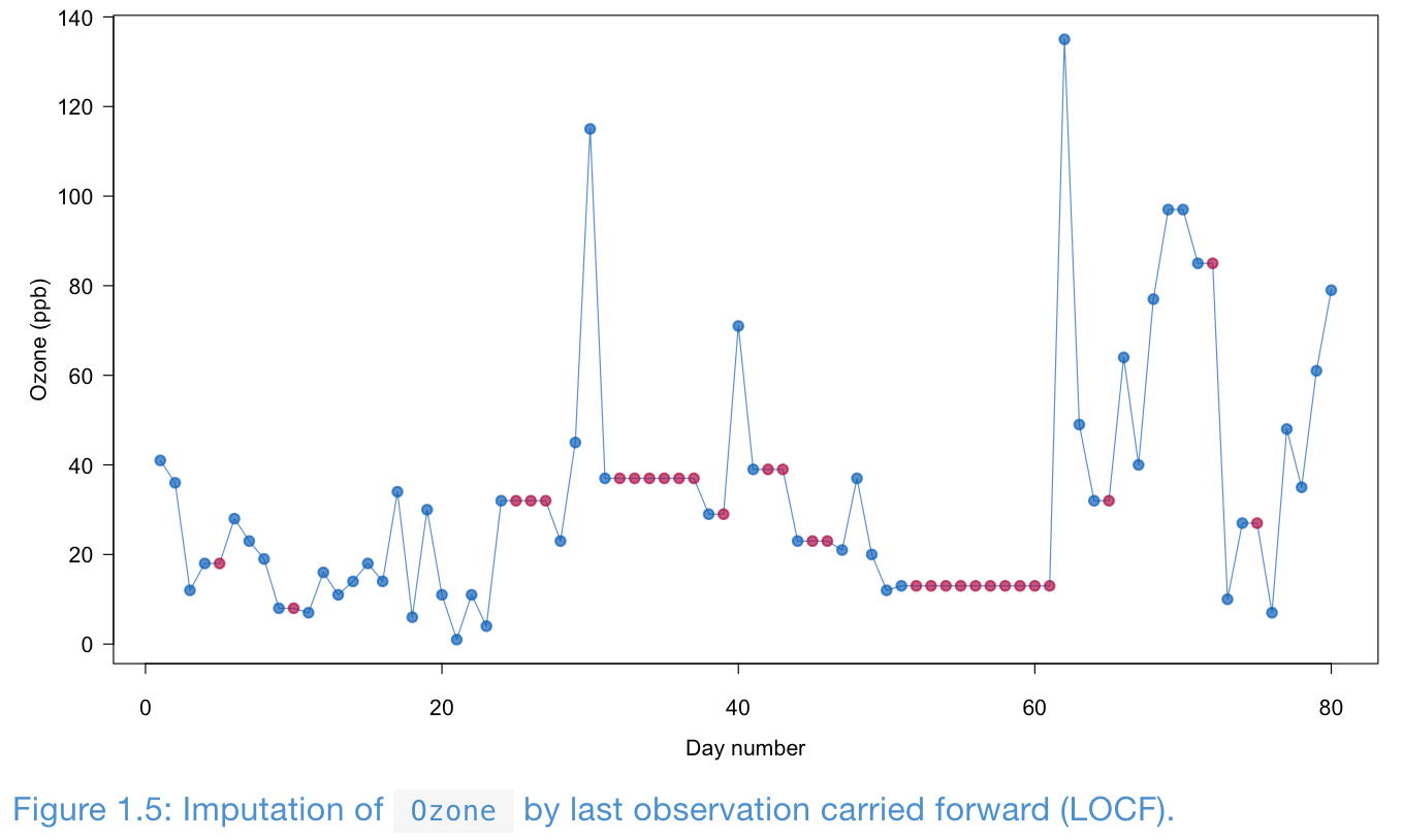
LOCF and BOCF
Last observation carried forward (LOCF) and baseline observation carried forward (BOCF) are for longitudinal data.
LOCF can yield biased estimation even under MCAR.
Indicator method
- Not for imputation, but for building predictive models
- Only works for missing in covariates, not the target variables
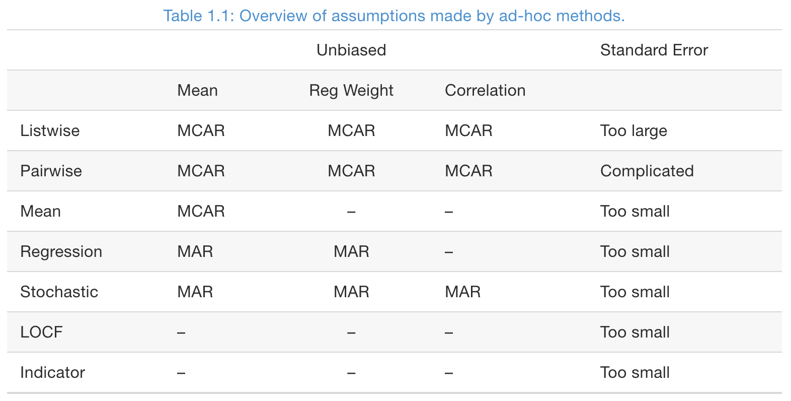
Summary of ad-hoc imputation methods
- Note: the unbiasness of regression coefficients are assess with the variable containing missing values as the target variable
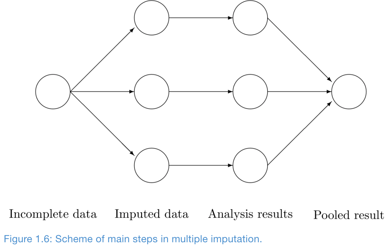
Multiple Imputation in a Nutshell
Multiple imputation creates \(m>1\) complete datasets
- Three steps of multiple imputation
- Imputation
- Analysis: train separate models
- Pooling: variance among \(m\) parameter estimates combines the conventional sampling variance (within-imputation variance) and the extra variance caused by the missing data (between-imputation variance)
Why using multiple imputation?
- It provides a mechanism to deal with the inherent uncertainty of the imputations
- It separate the solution of the missing data problem from the solution of the complete-data problem (train predictive models on complete data)
Multiple imputation example using the mice package
## Load the mice package
library(mice);
## Impute 20 times, using preditive mean matching
imp <- mice(airquality, seed = 1, m = 20, print = FALSE)
## Fit linear regressions
fit <- with(imp, lm(Ozone ~ Wind + Temp + Solar.R))
## Pooled regression estimates
pander(summary(pool(fit)))| term | estimate | std.error | statistic | df | p.value |
|---|---|---|---|---|---|
| (Intercept) | -60.21 | 21.57 | -2.791 | 100.3 | 0.006 |
| Wind | -3.174 | 0.644 | -4.927 | 83.29 | 0 |
| Temp | 1.584 | 0.228 | 6.959 | 125.7 | 0 |
| Solar.R | 0.058 | 0.023 | 2.454 | 79.63 | 0.016 |
References
Van Buuren, S. (2018). Flexible Imputation of Missing Data, 2nd Edition. CRC press.