Classical (Before Computer Age) Multiple Testing Corrections
- Bonferroni Correction
- Family-wise Error Rate
False Discovery Rates
- Benjamini-Hochberg FDR control
- An empirical Bayes view
Local False Discovery Rates
Empirical Null

For the pdf slides, click here

Classical (Before Computer Age) Multiple Testing Corrections

Background and notations

Before computer age, multiple testing may only involve 10 or 20 tests. With the emerge of biomedical (microarray) data, multiple testing may need to evaluate several thousands of tests
Notations
- $N$ : total number of tests, e.g., number of genes.
- $z_{i}$ : the z-statistic of the $i$ -th test. Note that if we perform tests other than z-test, say a t-test, then we can use inverse-cdf method to transform the t-statistic into a z-statistic, like below $z_{i} = Φ^{- 1} [F_{d f} (t_{i})],$ where $Φ$ is the standard normal cdf, and $F$ is a t distribution cdf.
- $I_{0}$ : the indices of the true $H_{0 i}$ , having $N_{0}$ members. Usually, majority of hypotheses are null, so $π_{0} = N_{0} / N$ is close to 1.
Hypotheses: standard normal vs normal with a non-zero mean $H_{0 i} : z_{i} \sim N (0, 1) ⟷ H_{1 i} : z_{i} \sim N (μ_{i}, 1)$ where $μ_{i}$ is the effect size for test $i$

Example: the prostate data

A microarray data of
- $n = 102$ people, 52 prostate cancer patients and 50 normal controls
- $N = 6033$ genes

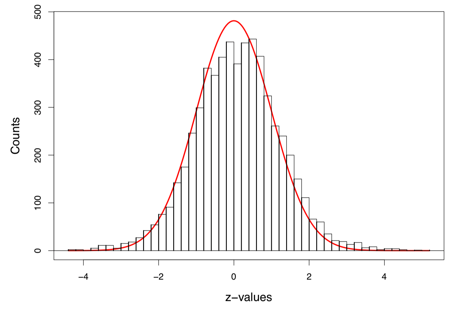
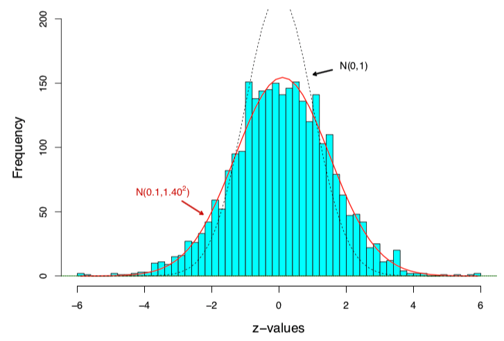
Figure 1: Histogram of 6033 z-values, with the scaled standard normal density curve in red

Bonferroni Correction

Classical multiple testing method 1: Bonferroni bound

For an overall significance level $α$ (usually $α = 0.05$ ), with $N$ simultaneous tests, the Bonferroni bound rejects the $i$ th null hypothesis $H_{0 i}$ at individual significance level

$p_{i} \leq \frac{α}{N}$

Bonferroni bound is quite conservative!
- For prostate data $N = 6033$ and $α = 0.05$ , the $p$ -value rejection cutoff is very small: $p_{i} \leq 8.3 \times 10^{- 6}$

Family-wise Error Rate

Classical multiple testing method 2: FWER control

The family-wise error rate is the probability of making even one false rejection $FWER = P (reject any true H_{0 i})$
Bonferroni’s procedure controls FWER, i.e., Bonferroni bound is more conservative than FWER control $\begin{aligned} FWER & = P {\cup_{i \in I_{0}} (p_{i} \leq \frac{α}{N})} \leq \sum_{i \in I_{0}} P (p_{i} \leq \frac{α}{N}) \\ = N_{0} \frac{α}{N} \leq α \end{aligned}$

FWER control: Holm’s procedure

Order the observed $p$ -values from smallest to largest $p_{(1)} \leq p_{(2)} \leq \dots \leq p_{(i)} \dots \leq p_{(N)}$
Reject null hypotheses $H_{0 (i)}$ if $p_{(i)} \leq Threshold(Holm's) = \frac{α}{N - i + 1}$

FWER is usually still too conservative for large $N$ , since it was originally developed for $N \leq 20$

An R function to implement Holm’s procedure

## A function to obtain Holm's procedure p-value cutoff
holm = function(pi, alpha=0.1){
  N = length(pi)
  idx = order(pi)
  reject = which(pi[idx] <= alpha/(N - 1:N + 1))
  
  return(idx[reject])
}

## Download prostate data's z-values
link = 'https://web.stanford.edu/~hastie/CASI_files/DATA/prostz.txt'
prostz = c(read.table(link))$V1
## Convert to p-values
prostp = 1 - pnorm(prostz)

Illustrate Holm’s procedure on the prostate data

## Apply Holm's procedure on the prostate data
results = holm(prostp)
## Total number of rejected null hypotheses
r = length(results); r

## [1] 6

## The largest z-value among non-rejected nulls
sort(prostz, decreasing = TRUE)[r + 1]

## [1] 4.13538

## The smallest p-value among non-rejected nulls
sort(prostp)[r + 1]

## [1] 1.771839e-05

False Discovery Rates

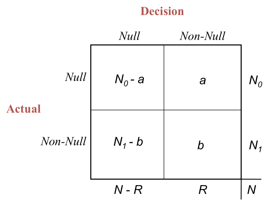
False discovery proportion

FDR control is a more liberal criterion (compared with FWER), thus it has become standard for large $N$ multiple testing problems.
False discovery proportion $Fdp (D) = {\begin{cases} a / R, & if R \neq 0 \\ 0, & if R = 0 \end{cases}$
- A decision rule $D$ rejects $R$ out of $N$ null hypotheses
- $a$ of those are false discoveries (unobservable)

False discovery rate

False discovery rates $FDR (D) = E {Fdp (D)}$
A decision rule $D$ controls FDR at level $q$ , if $FDR (D) \leq q$
- $q$ is a prechosen value between 0 and 1

Benjamini-Hochberg FDR control

Order the observed $p$ -values from smallest to largest $p_{(1)} \leq p_{(2)} \leq \dots \leq p_{(i)} \dots \leq p_{(N)}$
Reject null hypotheses $H_{0 (i)}$ if $p_{(i)} \leq Threshold (D_{q}) = \frac{q}{N} i$

Default choice $q = 0.1$
Theorem: if the $p$ -values are independent of each other, then the above procedure controls FDR at level $q$ , i.e., $FDR (D_{q}) = π_{0} q \leq q, where π_{0} = N_{0} / N$
- Usually, majority of the hypotheses are truly null, so $π_{0}$ is near 1

An R function to implement Benjamini-Hochberg FDR control

## A function to obtain Holm's procedure p-value cutoff
bh = function(pi, q=0.1){
  N = length(pi)
  idx = order(pi)
  reject = which(pi[idx] <= q/N * (1:N))
  
  return(idx[reject])
}

Illustrate Benjamini-Hochberg FDR control on the prostate data

## Apply Holm's procedure on the prostate data
results = bh(prostp)
## Total number of rejected null hypotheses
r = length(results); r

## [1] 28

## The largest z-value among non-rejected nulls
sort(prostz, decreasing = TRUE)[r + 1]

## [1] 3.293507

## The smallest p-value among non-rejected nulls
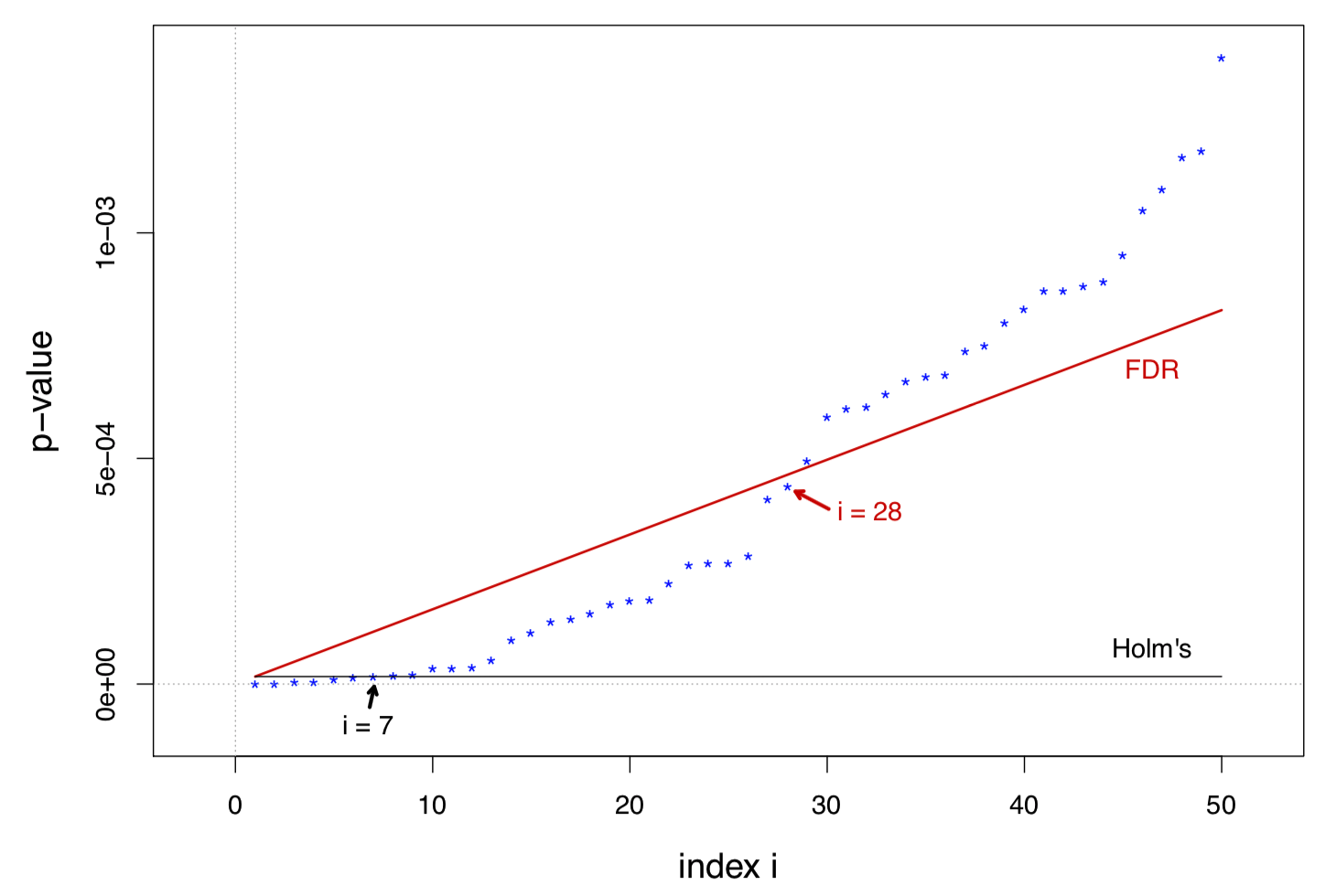
sort(prostp)[r + 1]

## [1] 0.0004947302

Comparing Holm’s FWER control and Benjamini-Hochberg FDR control

In the usual range of interest, large $N$ and small $i$ , the ratio $\frac{Threshold (D_{q})}{Threshold(Holm's)} = \frac{q}{α} (1 - \frac{i - 1}{N}) i$ increases with $i$ almost linearly
The figure below is about the prostate data, with $α = q = 0.1$

Question about the FDR control procedure

Is controlling a rate (i.e., FDR) as meaningful as controlling a probability (of Type 1 error)?
How should $q$ be chosen?
The control theorem depends on independence among the $p$ -values. What if they’re dependent, which is usually the case?
The FDR significance for one gene depends on the results of all other genes. Does this make sense?

An empirical Bayes view

Two-groups model

Each of the $N$ cases (e.g., genes) is
- either null with prior probability $π_{0}$ ,
- or non-null with probability $π_{1} = 1 - π_{0}$
For case $i$ , its $z$ -value $z_{i}$ under $H_{i j}$ for $j = 0, 1$ has density $f_{j} (z)$ , cdf $F_{j} (z)$ , and survival curve $S_{j} (z) = 1 - F_{j} (z)$
The mixture survival curve $\begin{aligned} S (z) = π_{0} S_{0} (z) + π_{1} S_{1} (z) \end{aligned}$

Bayesian false-discovery rate

Suppose the observation $z_{i}$ for case $i$ is seen to exceed some threshold value $z_{0}$ (say $z_{0} = 3$ ). By Bayes’ rule, the Bayesian false-discovery rate is $\begin{aligned} Fdr (z_{0}) & = P (case i is null ∣ z_{i} \geq z_{0}) \\ = \frac{π_{0} S_{0} (z_{0})}{S (z_{0})} \end{aligned}$
The “empirical” Bayes reflects in the estimation of the denominator: when $N$ is large, $\hat{S} (z_{0}) = \frac{N (z_{0})}{N}, N (z_{0}) = # {z_{i} \geq z_{0}}$
An empirical Bayes estimate of the Bayesian false-discovery rate $\hat{Fdr} (z_{0}) = \frac{π_{0} S_{0} (z_{0})}{\hat{S} (z_{0})}$

Connection between $\hat{Fdr}$ and FDR controls

Since $p_{i} = S_{0} (z_{i})$ and $\hat{S} (z_{(i)}) = i / N$ , the FDR control $D_{q}$ algorithm $p_{(i)} \leq \frac{i}{N} \cdot q$ becomes $S_{0} (z_{(i)}) \leq \hat{S} (z_{(i)}) \cdot q,$ After rearranging the above formula, we have its Bayesian Fdr bounded $\hat{Fdr} (z_{0}) \leq π_{0} q$
The FDR control algorithm is in fact rejecting those cases for which the empirical Bayes posterior probability of nullness is too small

Answer the 4 questions about the FDR control

(Rate vs probability) FDR control does relate to the posterior probability of nullness
(Choice of $q$ ) We can set $q$ according to the maximum tolerable amount of Bayes risk of nullness, usually after taking $π_{0} = 1$ in
(Independence) Most often the $z_{i}$ , and hence the $p_{i}$ , are correlated. However even under correlation, $\hat{S} (z_{0})$ is still an unbiased estimator for $S_{(} z_{0})$ , making $\hat{Fdr} (z_{0})$ nearly unbiased for $Fdr (z_{0})$ .
- There is a price to be paid for correlation, which increases the variance of $\hat{S} (z_{0})$ and $\hat{Fdr} (z_{0})$
(Rejecting one test depending on others) In the Bayes two-group model, the number of null cases $z_{i}$ exceeding some threshold $z_{0}$ has fixed expectation $N π_{0} S_{0} (z_{0})$ . So an increase in the number of $z_{i}$ exceeding $z_{0}$ must come from a heavier right tail for $f_{1} (z)$ , implying a greater posterior probability of non-nullness $Fdr (z_{0})$ .
- This emphasizes the “learning from the experience of others” aspect of empirical Bayes inference

Local False Discovery Rates

Local false discovery rates

Having observed test statistic $z_{i}$ equal to some value $z_{0}$ , we should be more interested in the probability of nullness given $z_{i} = z_{0}$ than $z_{i} \geq z_{0}$
Local false discovery rate $\begin{aligned} fdr (z_{0}) & = P (case i is null ∣ z_{i} = z_{0}) \\ = \frac{π_{0} f_{0} (z_{0})}{f (z_{0})} \end{aligned}$
After drawing a smooth curve $\hat{f} (z)$ through the histogram of the $z$ -values, we get the estimate $\hat{fdr} (z_{0}) = \frac{π_{0} f_{0} (z_{0})}{\hat{f} (z_{0})}$
- the null proportion $π_{0}$ can either be estimated or set equal to 1

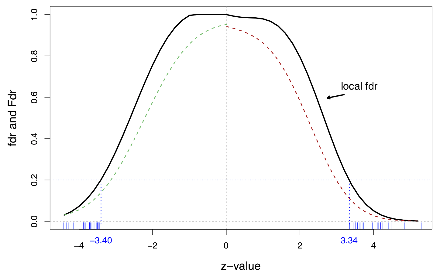
A fourth-degree log polynomial Poisson regression fit to the histogram, on the prostate data

Solid line is the local $\hat{fdr} (z)$ and dashed lines are tail-area $\hat{Fdr} (z)$
27 genes on the right and 25 one the left have $\hat{fdr} (z_{i}) \leq 0.2$

The default cutoff for local fdr

The cutoff $\hat{fdr} (z_{i}) \leq 0.2$ is equivalent to $\frac{f_{1} (z)}{f_{0} (z)} \geq 4 \frac{π_{0}}{π_{1}}$
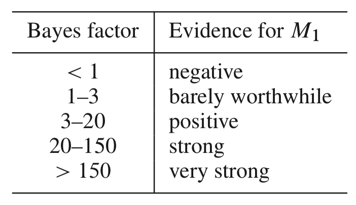
Assuming $π_{0} \geq 0.9$ , this makes the factor factor quite large $\frac{f_{1} (z)}{f_{0} (z)} \geq 36$ This is “strong evidence” against the null hypothesis in Jeffrey’s scale of evidence for the interpretation of Bayes factors

Relation between the local and tail-area fdr’s

Since $Fdr (z_{0}) = E (fdr (z) ∣ z \geq z_{0})$ Therefore $Fdr (z_{0}) < fdr (z_{0})$
Thus, the conventional significant cutoffs are $\begin{aligned} \hat{Fdr} (z) & \leq 0.1 \\ \hat{fdr} (z) & \leq 0.2 \end{aligned}$

Empirical Null

Empirical null

Large scale applications may allow us to empirically determine a more realistic null distribution than $H_{0 i} : z_{i} \sim N (0, 1)$
In the police data, a $N (0, 1)$ curve is too narrow for the null. Actually, an MLE fit to central data gives $N (0.10, {1.40}^{2})$ as the empirical null

Empirical null estimation

The theoretical null $z_{i} \sim N (0, 1)$ is not completely wrong, but needs adjustment for the dataset at hand
Under the two-group model, with $f_{0} (z)$ normal but not necessarily standard normal $f_{0} (z) \sim N (δ_{0}, σ_{0}^{2}),$ to compute the local $fdr (z) = π_{0} f_{0} (z) / f (z)$ , we need to estimate three parameters $(δ_{0}, σ_{0}, π_{0})$
Our key assumption is that $π_{0}$ is large, say $π_{0} \geq 0.9$ , and most of the $z_{i}$ near $0$ are null.
The algorithm locfdr begins by selecting a set $A_{0}$ near $z = 0$ and assumes that all the $z_{i}$ in $A_{0}$ are null
Maximum likelihood based on the numbers and values of $z_{i}$ in $A_{0}$ yield the empirical null estimates $({\hat{δ}}_{0}, {\hat{σ}}_{0}, {\hat{π}}_{0})$

References

Efron, Bradley and Hastie, Trevor (2016), Computer Age Statistical Inference. Cambridge University Press
Links to the prostate data
- The $6033 \times 102$ data matrix: prostmat.csv
- The $6033$ z-values: prostz.txt
A list of FDR methods in R: http://www.strimmerlab.org/notes/fdr.html

Book Notes: Computer Age Statistical Inference -- Ch15 Multiple Testing

Classical (Before Computer Age) Multiple Testing Corrections

Background and notations

Example: the prostate data

Bonferroni Correction

Classical multiple testing method 1: Bonferroni bound

Family-wise Error Rate

Classical multiple testing method 2: FWER control

FWER control: Holm’s procedure

An R function to implement Holm’s procedure

Illustrate Holm’s procedure on the prostate data

False Discovery Rates

False discovery proportion

False discovery rate

Benjamini-Hochberg FDR control

Benjamini-Hochberg FDR control

An R function to implement Benjamini-Hochberg FDR control

Illustrate Benjamini-Hochberg FDR control on the prostate data

Comparing Holm’s FWER control and Benjamini-Hochberg FDR control

Question about the FDR control procedure

An empirical Bayes view

Two-groups model

Bayesian false-discovery rate

Connection between ˆFdrFdr^ and FDR controls

Answer the 4 questions about the FDR control

Local False Discovery Rates

Local false discovery rates

A fourth-degree log polynomial Poisson regression fit to the histogram, on the prostate data

The default cutoff for local fdr

Relation between the local and tail-area fdr’s

Empirical Null

Empirical null

Empirical null estimation

References

Connection between $\hat{Fdr}$ and FDR controls