For the pdf slides, click here
Notations: in binary classification
We are interested in fitting a model \(q(\mathbf{x})\) for the true conditional class 1 probability \[ \eta(\mathbf{x}) = P(Y = 1 \mid \mathbf{X} = \mathbf{x}) \]
Two types of problems
- Classification: estimating a region of the form \(\{\eta(\mathbf{x}) > c\}\)
- Class probability estimation: approximate \(\eta(\mathbf{x})\), by fitting a model \(q(\mathbf{x}, \beta)\), where \(\beta\) are parameters to be estimated
Surrogate criteria for estimation, e.g.,
- Log-loss: \(L(y \mid q) = -y \log(q) - (1-y) \log (1-q)\)
- Squared error loss: \(L(y \mid q) = (y-q)^2 = y (1-q)^2 + (1-y) q^2\)
Surrogate criteria of classification are exactly the primary criteria of class probability estimation
Proper Scoring Rules
Proper scoring rule
Fitting a binary model is to minimize a loss function \[ \mathcal{L}\left(q()\right) = \frac{1}{N}\sum_{n=1}^N L(y_n \mid q_n) \]
In game theory, the agent’s goal is to maximize expected score (or minimize expected loss)
- A scoring rule is proper if truthfulness maximizes expected score
- It is strictly proper if truthfulness uniquely maximizes expected score
In the context of binary response data, Fisher consistency holds pointwise if \[ \arg\min_{q\in [0, 1]} E_{Y\sim \text{Bernoulli}(\eta)}L(Y\mid q) = \eta, \quad \forall \eta \in [0, 1] \]
Fisher consistency is the defining property of proper scoring rules
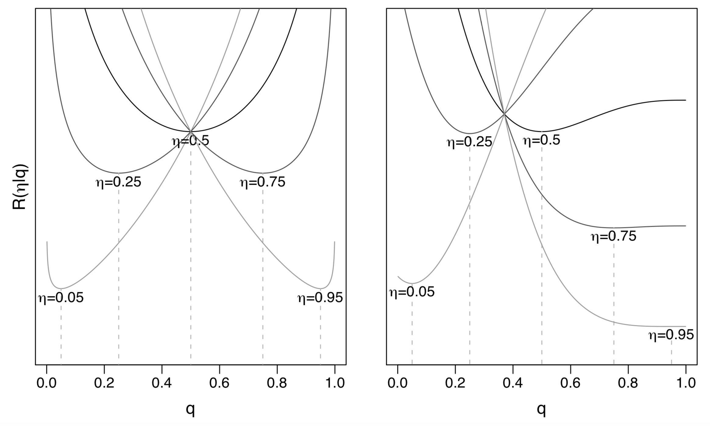
Visualization of two proper scoring rules
- Left: log-loss, or Beta loss with \(\alpha=\beta=0\)
Right: Beta loss with \(\alpha=1, \beta=3\)
- Tailored for classification with false positive cost \(c = \frac{\alpha}{\alpha+\beta} = 0.25\) and false negative cost \(1-c = 0.75\)
Commonly Used Proper Scoring Rules
How to check property of a scoring rule for binary response data
Suppose the partial losses \(L_1(1-q), L_0(q)\) are smooth, then the proper scoring rule property implies \[\begin{align*} 0 & = \left.\frac{\partial}{\partial q}\right|_{q=\eta} R(\eta \mid q)\\ & = -\eta L_1'(1-\eta) + (1-\eta) L_0'(\eta) \end{align*}\]
Therefore, a scoring rule is proper if \[ \eta L_1'(1-\eta) = (1-\eta) L_0'(\eta) \]
A scoring rule is strictly proper if \[ \left.\frac{\partial^2}{\partial q^2}\right|_{q=\eta} R(\eta \mid q) > 0 \]
Log-loss
Log-loss is the negative log likelihood of the Bernoulli distribution \[ \mathcal{L} = \frac{1}{N}\sum_{n=1}^N\left[-y_n \log(q_n) - (1-y_n) \log(1 - q_n) \right] \]
Partial losses for log-loss \[ L_1(1-q) = -\log(q), \quad L_0(q) = -\log(1-q) \]
Expected loss for log-loss \[ R(\eta \mid q) = -\eta \log(q) - (1-\eta)\log(1-q) \]
Log-loss is a strictly proper scoring rule
Squared error loss
Squared error loss is also known as Brier score \[ \mathcal{L} = \frac{1}{N}\sum_{n=1}^N\left[y_n (1 - q_n)^2 - (1-y_n)q_n^2 \right] \]
Partial losses for squared error loss \[ L_1(1-q) = (1 - q)^2, \quad L_0(q) = q^2 \]
Expected loss for squared error loss \[ R(\eta \mid q) = \eta (1 - q)^2 + (1-\eta)q^2 \]
Squared error loss is a strictly proper scoring rule
Misclassification loss
Usually, misclassification loss uses \(c=0.5\) as the cutoff \[ \mathcal{L} = \frac{1}{N}\sum_{n=1}^N\left[y_n \mathbf{1}_{\{q_n \leq 0.5\}} + (1-y_n)\mathbf{1}_{\{q_n > 0.5\}} \right] \]
Partial losses for misclassification loss \[ L_1(1-q) = \mathbf{1}_{\{q_n \leq 0.5\}}, \quad L_0(q) = \mathbf{1}_{\{q_n > 0.5\}} \]
Expected loss for misclassification loss \[ R(\eta \mid q) = \eta \mathbf{1}_{\{q \leq 0.5\}} + (1-\eta) \mathbf{1}_{\{q > 0.5\}} \]
Since any \(q>0.5\) for events and any \(q \leq 0.5\) for non-events minimize the misclassification loss, misclassification loss is a proper score rule, but it is not strictly proper
A counter-example of proper scoring rule: absolute loss
Because \(y\in \{0, 1\}\), the absolute deviation \(L(y\mid q) = |y-q|\) becomes \[\begin{align*} L(y\mid q) & = y(1-q) + (1-y) q\\ R(\eta \mid q)& =\eta(1-q) + (1-\eta) q \end{align*}\]
Absolute deviation is not a proper scoring rule, because \(R(\eta \mid q)\) is minimized by \(q=1\) for \(\eta > 1/2\), and \(q=0\) for \(\eta < 1/2\)
Structure of Proper Scoring Rules
Structure of proper scoring rules
Theorem: Let \(\omega(dt)\) be a positive measure on \((0, 1)\) that is finite on intervals \((\epsilon, 1-\epsilon), \forall \epsilon > 0\). Then the following defines a proper scoring rule: \[ L_1(1-q) = \int_q^{f_1} (1-t)\omega(dt), \quad L_0(q) = \int_{f_0}^q t\omega(dt) \]
The proper scoring rule is strict iff \(\omega(dt)\) has non-zero mass on every open interval of (0, 1)
The fixed limits \(f_0\geq 0\) and \(f_1 \leq 1\) are somewhat arbitrary
Note that for log-loss, \(L_1(1-q)\) is unbounded (goes to infinity) below near \(q=1\), and \(L_0(q)\) is unbounded below near \(q=0\)
Except for log-loss, all other common proper scoring rules seem to satisfy \[ \int_0^1 t (1-t) \omega(dt) < \infty \]
Proper scoring rules are mixtures of cost-weighted misclassification losses
Connection between the false positive (FP) / false negative (FN) costs and the classification cutoff
Suppose the costs of FP and FN sum up to 1:
- FP: has a cost \(c\), and expected cost \(c P(Y=0) = c(1-\eta)\)
- FN: has a cost \(1 - c\), and expected cost \((1-c) P(Y=1) = (1-c)\eta\)
The optimal classification is therefore class 1 iff \[ (1-c)\eta \geq c(1-\eta) \Longleftrightarrow \eta \geq c \]
- Since we don’t know the truth \(\eta\), we classify as class 1 when \(q \geq c\)
Therefore, the classification cutoff equals \[ \frac{\text{cost of FP}}{\text{cost of FP} + \text{cost of FN}} \]
- Standard classification assumes costs of FP and FN are the same, so the classification cutoff is \(0.5\)
Cost-weighted misclassification errors
Cost-weighted misclassification errors: \[\begin{align*} L_c(y\mid q) & = y (1-c) \cdot \mathbf{1}_{\{q \leq c\}} + (1-y) c \cdot \mathbf{1}_{\{q > c\}} \\ L_{1, c}(1-q) &= (1-c) \cdot \mathbf{1}_{\{q \leq c\}}, \quad L_{0, c}(q) = c \cdot \mathbf{1}_{\{q > c\}} \end{align*}\]
Shuford-Albert-Massengil-Savage-Schervish theorem: an intergral representation of proper scoring rules \[ L(y\mid q) = \int_0^1 L_c(y\mid q) \omega(dc) = \int_0^1 L_c(y\mid q) \omega(c) dc \]
- The second equality holds if \(w(dc)\) is absolutely continuous wrt Lebesgue measure
- This can be used to tailor losses to specific classification problems with cutoffs other than \(1/2\) of \(\eta(x)\), by designing suitable weight functions \(\omega()\)
The paper proposes to use Iterative Reweighted Least Squares (IRLS) to fit linear models with proper scoring rules
Beta Family of Proper Scoring Rules
Beta family of proper scoring rules
This paper introduced a flexible 2-parameter family of proper scoring rules \[ \omega(t) = t^{\alpha-1} (1-t)^{\beta-1}, \quad \text{where } \alpha > -1, \beta > -1 \]
Loss function of the Beta family proper scoring rules \[\begin{align*}L(y \mid q) =~& y \int_q^1 t^{\alpha-1} (1-t)^{\beta} dt + (1-y)\int_0^q t^{\alpha} (1-t)^{\beta-1} dt\\ =~& y B(\alpha, \beta+1) \left[1 - I_q(\alpha, \beta+1)\right]\\ & + (1-y) B(\alpha+1, \beta) I_q(\alpha+1, \beta) \end{align*}\]
- See the definitions of \(B(a, b)\) and \(I_x(a, b)\) in the next page
Log-loss and squared error loss are special cases
- Log-loss: \(\alpha=\beta=0\)
- Squared error loss: \(\alpha=\beta=1\)
- Misclassification loss: \(\alpha=\beta \rightarrow \infty\)
Special functions and Python / R implementations
Beta function \[ B(a, b) = \int_0^1 t^{a-1} (1-t)^{b-1} dt %= \frac{\Gamma(a) \Gamma(b)}{\Gamma(a+b)} \]
- Python implementation:
scipy.special.beta(a,b) - R implementation:
beta(a, b)
- Python implementation:
Incomplete Beta function \[\begin{align*} I_x(a, b) %& = \frac{\Gamma(a+b)}{\Gamma(a) \Gamma(b)}\int_0^x t^{a-1} (1-t)^{b-1} dt \\ & = \frac{1}{B(a, b)} \int_0^x t^{a-1} (1-t)^{b-1} dt \end{align*}\]
- Python implementation:
scipy.special.betainc(a, b, x) - R implementation:
pbeta(x, a, b)
- Python implementation:
Tailor proper scoring rules for cost-weighted misclassification
We can use \(\alpha\neq \beta\) when FP and FN costs are not viewed equal
Since Beta family proper scoring rule is like adding a Beta distribution on the FP cost \(c\), we can use mean/variance matching to elicit \(\alpha\) and \(\beta\) \[\begin{align*} \mu & = \frac{\alpha}{\alpha + \beta} = c\\ \sigma^2 &= \frac{\alpha\beta}{(\alpha + \beta)^2 (\alpha + \beta+1)} = \frac{c(1-c)}{\alpha + \beta+1} \end{align*}\]
Alternatively, we can match the mode \[ c = q_{\text{mode}} = \frac{\alpha-1}{\alpha+\beta -2} \]
Examples
A simulation example
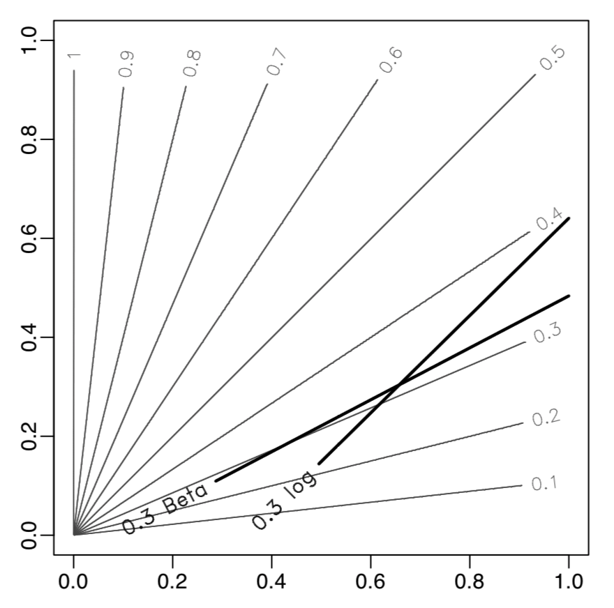
In the simulation data with bivariate \(x\), where decision boundaries of different \(\eta\) are not in parallel (grey lines)
The logit link Beta family linear model with \(\alpha = 6, \beta = 14\) estimates the \(c=0.3\) classification boundary better than the logistic regression
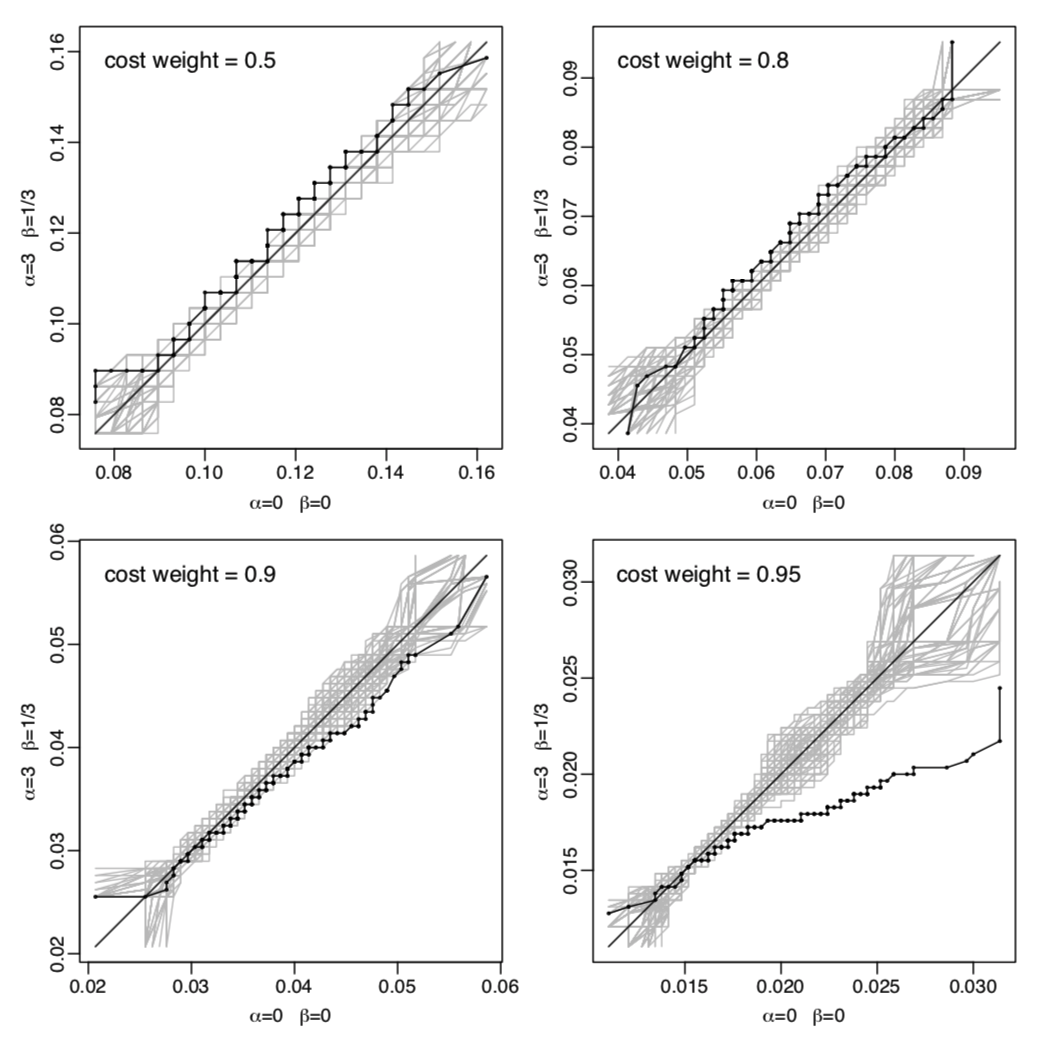
On the Pima Indians diabetes data
Comparing logistic regression with a proper scoring rule tailored for high class 1 probabilities: \(\alpha = 9, \beta = 1\).
Black lines: empirical QQ curves of 200 cost-weighted misclassification costs computed on randomly selected test sets
References
Buja, A., Stuetzle, W., & Shen, Y. (2005). Loss functions for binary class probability estimation and classification: Structure and applications. Working draft, November, 3. http://www-stat.wharton.upenn.edu/~buja/PAPERS/paper-proper-scoring.pdf
For a game theory definition of proper scoring rule, see https://www.cis.upenn.edu/~aaroth/courses/slides/agt17/lect23.pdf
Fitting linear models with custom loss functions in Python: https://alex.miller.im/posts/linear-model-custom-loss-function-regularization-python/
Fitting XGBoost with custom loss functions in Python: https://xgboost.readthedocs.io/en/latest/tutorials/custom_metric_obj.html