For the pdf slides, click here
Variational Inference
Introduction of the variational inference method
Definitions
- Variational inference is also called variational Bayes,
thus
- all parameters are viewed as random variables, and
- they will have prior distributions.
- We denote the set of all latent variables and parameters by \(\mathbf{Z}\)
- Note: the parameter vector \(\boldsymbol\theta\) no long appears, because it’s now a part of \(\mathbf{Z}\)
- Goal: find approximation for
- posterior distribution \(p(\mathbf{Z} \mid \mathbf{X})\), and
- marginal likelihood \(p(\mathbf{X})\), also called the model evidence
Model evidence equals lower bound plus KL divergence
Goal: We want to find a distribution \(q(\mathbf{Z})\) that approximates the posterior distribution \(p(\mathbf{Z}\mid \mathbf{X})\). In other word, we want to minimize the KL divergence \(\text{KL}(q \| p)\).
Note the decomposition of the marginal likelihood \[ \log p(\mathbf{X}) = \mathcal{L}(q) + \text{KL}(q \| p), \]
Thus, maximizing the lower bound (also called ELBO) \(\mathcal{L}(q)\) is equivalent to minimizing the KL divergence \(\text{KL}(q \| p)\). \[\begin{align*} \mathcal{L}(q) & = \int q(\mathbf{Z}) \log\left\{ \frac{p(\mathbf{X}, \mathbf{Z})}{q(\mathbf{Z})} \right\} d\mathbf{Z}\\ \text{KL}(q \| p) & = -\int q(\mathbf{Z}) \log\left\{ \frac{p(\mathbf{Z}\mid \mathbf{X})}{q(\mathbf{Z})} \right\} d\mathbf{Z} \end{align*}\]
Mean field family
Goal: restrict the family of distribution \(q(\mathbf{Z})\) so that they comprise only tractable distributions, while allow the family to be sufficiently flexible so that it can approximate the posterior distribution well
- Mean field family : partition the elements of \(\mathbf{Z}\) into disjoint groups
denoted by \(\mathbf{Z}_j\), for \(j = 1, \ldots, M\), and assume \(q\) factorizes wrt these groups:
\[
q(\mathbf{Z}) = \prod_{j=1}^M q_j(\mathbf{Z}_j)
\]
- Note: we place no resitriction on the functional forms of the individual factors \(q_j(\mathbf{Z}_j)\)
Solution for mean field families: derivation
We will optimize wrt each \(q_j(\mathbf{Z}_j)\) in turn.
For \(q_j\), the lower bound (to be maximized) can be decomposed as \[\begin{align*} \mathcal{L}(q) & = \int \prod_k q_k \left\{\log p(\mathbf{X}, \mathbf{Z}) - \sum_k \log q_k \right\}d\mathbf{Z}\\ & = \int q_j \underbrace{\left\{\int \log p(\mathbf{X}, \mathbf{Z}) \prod_{k\neq j} q_k d\mathbf{Z}_k\right\}}_{\mathbb{E}_{k\neq j}\left[ \log p(\mathbf{X}, \mathbf{Z}) \right]} d\mathbf{Z}_j - \int q_j \log q_j d\mathbf{Z}_j + \text{const}\\ & = -\text{KL}\left(q_j \| \tilde{p}(\mathbf{X}, \mathbf{Z}_j) \right) + \text{const} \end{align*}\]
- Here the new distribution \(\tilde{p}(\mathbf{X}, \mathbf{Z}_j)\) is defined as \[ \log \tilde{p}(\mathbf{X}, \mathbf{Z}_j) = \mathbb{E}_{k\neq j}\left[ \log p(\mathbf{X}, \mathbf{Z}) \right] + \text{const} \]
Solution for mean field families
A general expression for the optimal solution \(q_j^*(\mathbf{Z}_j)\) is \[ \log q_j^*(\mathbf{Z}_j) = \mathbb{E}_{k\neq j}\left[ \log p(\mathbf{X}, \mathbf{Z})\right] + \text{const} \]
- We can only use this solution in an iterative manner, because the expectations should be computed wrt other factors \(q_k(\mathbf{Z}_k)\) for \(k \neq j\).
- Convergence is guaranteed because bound is convex wrt each factor \(q_j\)
- On the right hand side we only need to retain those terms that have some functional dependence on \(\mathbf{Z}_j\)
Example: approximate a bivariate Gaussian using two independent distributions
Target distribution: a bivariate Gaussian \[ p(\mathbf{z}) = \text{N}\left(\mathbf{z} \mid \boldsymbol\mu, \boldsymbol\Lambda^{-1}\right), \quad \boldsymbol\mu = \left( \begin{array}{c} \mu_1 \\ \mu_2 \end{array} \right), \quad \boldsymbol\Lambda = \left( \begin{array}{cc} \lambda_{11}& \lambda_{12}\\ \lambda_{12}& \lambda_{22} \end{array} \right) \]
We use a factorized form to approximate \(p(\mathbf{z})\): \[ q(\mathbf{z}) = q_1(z_1) q_2(z_2) \]
Note: we do not assume any functional forms for \(q_1\) and \(q_2\)
VI solution to the bivariate Gaussian problem
\[\begin{align*} \log q_1^*(z_1) &= \mathbb{E}_{z_2}\left[\log p(\mathbf{z})\right] + \text{const}\\ &= \mathbb{E}_{z_2}\left[ -\frac{1}{2}(z_1 - \mu_1)^2 \Lambda_{11} - (z_1 - \mu_1) \Lambda_{12} (z_2 - \mu_2) \right] + \text{const}\\ &= -\frac{1}{2}z_1^2 \Lambda_{11} + z_1 \mu_1 \Lambda_{11} - (z_1 - \mu_1) \Lambda_{12} \left(\mathbb{E}[z_2] - \mu_2\right) + \text{const} \end{align*}\]
Thus we identify a normal, with mean depending on \(\mathbb{E}[z_2]\): \[ q^*(z_1) = \text{N}\left(z_1 \mid m_1, \Lambda_{11}^{-1} \right), \quad m_1 = \mu_1 - \Lambda_{11}^{-1}\Lambda_{12}\left(\mathbb{E}[z_2] - \mu_2\right) \]
By symmetry, \(q^*(z_2)\) is also normal; its mean depends on \(\mathbb{E}[z_1]\) \[ q^*(z_2) = \text{N}\left(z_2 \mid m_2, \Lambda_{22}^{-1} \right), \quad m_2 = \mu_2 - \Lambda_{22}^{-1}\Lambda_{12}\left(\mathbb{E}[z_1] - \mu_1\right) \]
We treat the above variational solutions as re-estimation equations, and cycle through the variables in turn updating them until some convergence criterion is satisfied
Visualize VI solution to bivariate Gaussian
Variational inference minimizes KL\((q \| p)\): mean of the approximation is correct, but variance (along the orthogonal direction) is significantly under-estimated
Expectation propagation minimizes KL\((p \| q)\): solution equals marginal distributions
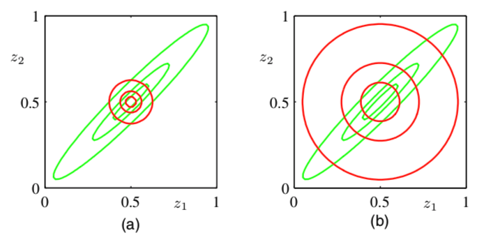
Figure 1: Left: variational inference. Right: expectation propagation
Another example to compare KL\((q \| p)\) and KL\((p \| q)\)
- To approximate a mixture of two Gaussians \(p\) (blue contour)
- Use a single Gaussian \(q\) (red contour) to approximate \(p\)
- By minimizing KL\((p\| q)\): figure (a)
- By minimizing KL\((q\| p)\): figure (b) and (c) show two local minimum
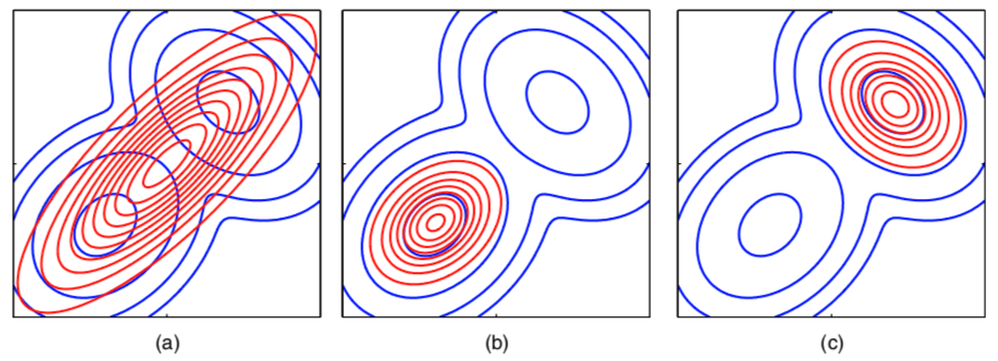
- For multimodal distribution
- a variational solution will tend to find one of the modes,
- but an expectation propagation solution would lead to poor predictive distribution (because the average of the two good parameter values is typically itself not a good parameter value)
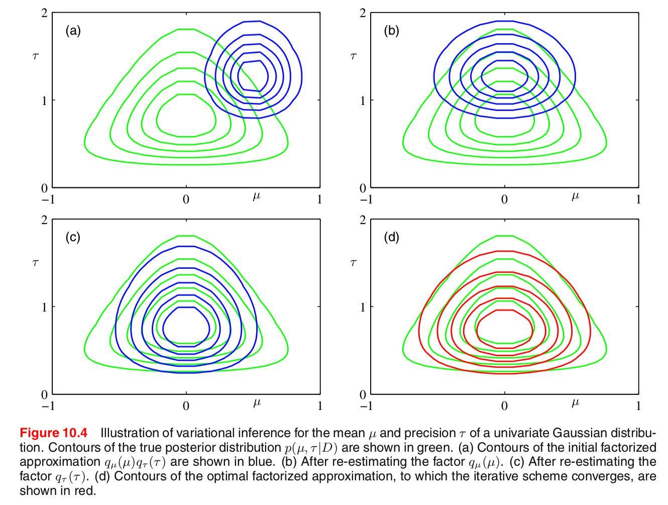
Example: univariate Gaussian
Example: univariate Gaussian
Suppose the data \(D = \{x_1, \ldots, x_N\}\) follows iid normal distribution \[ x_i \sim \text{N}\left(\mu, \tau^{-1}\right) \]
The prior distributions are \[\begin{align*} \mu \mid \tau & \sim \text{N}\left(\mu_0, (\lambda_0 \tau)^{-1}\right)\\ \tau & \sim \text{Gam}(a_0, b_0) \end{align*}\]
Factorized variational approximation \[ q(\mu, \tau) = q(\mu) q(\tau) \]
Variational solution for \(\mu\)
\[\begin{align*} \log q^*(\mu) &= \mathbb{E}_\tau\left[\log p(D \mid \mu, \tau) + \log p(\mu \mid \tau) \right] + \text{const}\\ &= -\frac{\mathbb{E}[\tau]}{2}\left\{ \lambda_0 (\mu - \mu_0)^2 + \sum_{i=1}^N (x_i - \mu)^2\right\}+ \text{const} \end{align*}\]
Thus, the variational solution for \(\mu\) is \[\begin{align*} q(\mu) &= \text{N}\left(\mu \mid \mu_N, \lambda_N^{-1}\right)\\ \mu_N &= \frac{\lambda_0 \mu_0 + N \bar{x}}{\lambda_0 + N}\\ \lambda_N &= \left(\lambda_0 + N\right)\mathbb{E}[\tau] \end{align*}\]
Variational solution for \(\tau\)
\[\begin{align*} \log q^*(\tau) &= \mathbb{E}_\mu\left[\log p(D \mid \mu, \tau) + \log p(\mu \mid \tau) + \log p(\tau)\right] + \text{const}\\ &= (a_0 -1)\log \tau - b_0 \tau + \frac{N}{2}\log \tau\\ &~~~~ - \frac{\tau}{2} \mathbb{E}_\mu\left[\lambda_0 (\mu - \mu_0)^2 + \sum_{i=1}^N (x_i - \mu)^2\right]+ \text{const} \end{align*}\]
Thus, the variational solution for \(\tau\) is \[\begin{align*} q(\tau) &= \text{Gam}\left(\tau \mid a_N, b_N\right)\\ a_N &= a_0 + + \frac{N}{2}\\ b_N &= b_0 + \frac{1}{2} \mathbb{E}_\mu\left[\lambda_0 (\mu - \mu_0)^2 + \sum_{i=1}^N (x_i - \mu)^2\right] \end{align*}\]
Visualization of VI solution to univariate normal
Model selection
Model selection (comparison) under variational inference
In addition to making inference on the parameter \(\mathbf{Z}\), we may also want to compare a set of candidate models, denoted by index \(m\)
We should consider the factorization \[ q(\mathbf{Z}, m) = q(\mathbf{Z} \mid m) q(m) \] to approximate the posterior \(p(\mathbf{Z}, m \mid \mathbf{X})\)
We can maximize the information lower bound \[ \mathcal{L}_m = \sum_m \sum_{\mathbf{Z}} q(\mathbf{Z} \mid m) q(m) \log\left\{\frac{p(\mathbf{Z}, \mathbf{X}, m)}{q(\mathbf{Z} \mid m) q(m) }\right\} \] which is a lower bound of \(\log p(\mathbf{X})\)
The maximized \(q(m)\) can be used for model selection
Variational Mixture of Gaussians
Mixture of Gaussians
For each observation \(\mathbf{x}_n \in \mathbb{R}^D\), we have a corresponding latent variable \(\mathbf{z}_n\), a 1-of-\(K\) binary group indicator vector
Mixture of Gasussians joint likelihood, based on \(N\) observations \[\begin{align*} p(\mathbf{Z} \mid \boldsymbol\pi) & = \prod_{n=1}^N \prod_{k=1}^K \pi_k^{z_{nk}}\\ p(\mathbf{X} \mid \mathbf{Z}, \boldsymbol\mu, \boldsymbol\Lambda) &= \prod_{n=1}^N \prod_{k=1}^K \text{N}\left(\mathbf{x}_n \mid \boldsymbol\mu_k, \boldsymbol\Lambda_k^{-1} \right)^{z_{nk}} \end{align*}\]
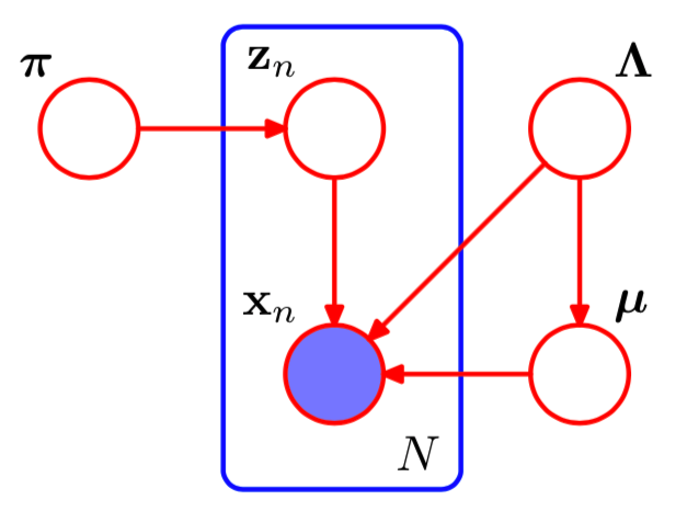
Figure 2: Graph representation of mixture of Gaussians
Conjugate priors
Dirichlet for \(\boldsymbol\pi\) \[ p(\boldsymbol\pi) = \text{Dir}(\boldsymbol\pi \mid \boldsymbol\alpha_0) \propto \prod_{k=1}^K \pi_k^{\alpha_{0k} - 1} \]
Independent Gaussian-Wishart for \(\boldsymbol\mu, \boldsymbol\Lambda\) \[\begin{align*} p(\boldsymbol\mu, \boldsymbol\Lambda) &= \prod_{k=1}^K p(\boldsymbol\mu_k \mid \boldsymbol\Lambda_k) p(\boldsymbol\Lambda_k)\\ &= \prod_{k=1}^K \text{N}\left(\boldsymbol\mu_k \mid \mathbf{m}_0, (\beta_0 \boldsymbol\Lambda_k)^{-1}\right) \text{W}\left( \boldsymbol\Lambda_k \mid \mathbf{W}_0, \nu_0 \right) \end{align*}\]
- Usually, the prior mean \(\mathbf{m}_0 = \mathbf{0}\)
Variational distribution
Joint posterior \[ p(\mathbf{X}, \mathbf{Z}, \boldsymbol\pi, \boldsymbol\mu, \boldsymbol\Lambda) = p(\mathbf{X} \mid \mathbf{Z}, \boldsymbol\mu, \boldsymbol\Lambda) p(\mathbf{Z} \mid \boldsymbol\pi) p(\boldsymbol\pi) p(\boldsymbol\mu \mid \boldsymbol\Lambda)p(\boldsymbol\Lambda) \]
Variational distribution factorizes between the latent variables and the parameters \[\begin{align*} q(\mathbf{Z}, \boldsymbol\pi, \boldsymbol\mu, \boldsymbol\Lambda) & = q(\mathbf{Z}) q(\boldsymbol\pi, \boldsymbol\mu, \boldsymbol\Lambda)\\ & = q(\mathbf{Z}) q(\boldsymbol\pi) \prod_{k=1}^K q(\boldsymbol\mu_k, \boldsymbol\Lambda_k) \end{align*}\]
Variational solution for \(\mathbf{Z}\)
Optimized factor \[\begin{align*} \log q^*(\mathbf{Z}) &= \mathbb{E}_{\boldsymbol\pi, \boldsymbol\mu, \boldsymbol\Lambda} \left[\log p(\mathbf{X}, \mathbf{Z}, \boldsymbol\pi, \boldsymbol\mu, \boldsymbol\Lambda) \right]\\ &= \mathbb{E}_{\boldsymbol\pi}\left[\log p(\mathbf{Z} \mid \boldsymbol\pi) \right] + \mathbb{E}_{\boldsymbol\mu, \boldsymbol\Lambda} \left[\log p(\mathbf{X} \mid \mathbf{Z}, \boldsymbol\mu, \boldsymbol\Lambda) \right]\\ &= \sum_{n=1}^N \sum_{k=1}^K z_{nk} \log \rho_{nk} + \text{const}\\ \log \rho_{nk} = ~& \mathbb{E}\left[\log \pi_{k}\right] + \frac{1}{2} \mathbb{E}\left[\log \left|\boldsymbol\Lambda_k \right| \right] - \frac{D}{2} \log(2\pi)\\ & - \frac{1}{2} \mathbb{E}_{\boldsymbol\mu, \boldsymbol\Lambda} \left[\left(\mathbf{x}_n - \boldsymbol\mu_k\right)' \Lambda_k \left(\mathbf{x}_n - \boldsymbol\mu_k\right) \right] \end{align*}\]
Thus, the factor \(q^*(\mathbf{Z})\) takes the same functional form as the prior \(p(\mathbf{Z} \mid \boldsymbol\pi)\) \[ q^*(\mathbf{Z}) = \prod_{n=1}^N \prod_{k=1}^K r_{nk}^{z_{nk}}, \quad r_nk = \frac{\rho_{nk}}{\sum_{j=1}^K \rho_{nj}} \]
- By \(q^*(\mathbf{Z})\), the posterior mean (i.e., responsibility) \(\mathbb{E}[z_{nk}] = r_{nk}\)
Define three statistics wrt the responsibilities
- For each of group \(k = 1, \ldots, K\), denote \[\begin{align*} N_k & = \sum_{n=1}^N r_{nk}\\ \bar{\mathbf{x}}_k &= \frac{1}{N_k} \sum_{n=1}^N r_{nk} \mathbf{x}_n\\ \mathbf{S}_k &= \frac{1}{N_k} \sum_{n=1}^N r_{nk} \left(\mathbf{x}_n - \bar{\mathbf{x}}_k\right) \left(\mathbf{x}_n - \bar{\mathbf{x}}_k\right)' \end{align*}\]
Variational solution for \(\boldsymbol\pi\)
Optimized factor \[\begin{align*} \log q^*(\boldsymbol\pi) &= \log p(\boldsymbol\pi) + \mathbb{E}_{\mathbf{Z}}\left[ p(\mathbf{Z} \mid \boldsymbol\pi) \right]\\ &= (\alpha_0 -1) \sum_{k=1}^K \log \pi_k + \sum_{k=1}^K \sum_{n=1}^N r_{nk} \log \pi_{nk} + \text{const} \end{align*}\]
Thus, \(q^*(\boldsymbol\pi)\) is a Dirichlet distribution \[ q^*(\boldsymbol\pi) = \text{Dir}(\boldsymbol\alpha), \quad \alpha_k = \alpha_0 + N_k \]
Variational solution for \(\boldsymbol\mu_k, \boldsymbol\Lambda_k\)
Optimized factor for \((\boldsymbol\mu_k, \boldsymbol\Lambda_k)\) \[\begin{align*} \log q^*(\boldsymbol\mu_k, \boldsymbol\Lambda_k) =~& \mathbb{E}_{\mathbf{Z}}\left[ \sum_{n=1}^N z_{nk} \log \text{N}\left(\mathbf{x}_n \mid \boldsymbol\mu_k, \boldsymbol\Lambda_k^{-1} \right) \right]\\ & + \log p(\boldsymbol\mu_k \mid \boldsymbol\Lambda_k) + \log p(\boldsymbol\Lambda_k) \end{align*}\]
Thus, \(q^*(\boldsymbol\mu_k, \boldsymbol\Lambda_k)\) is Gaussian-Wishart \[\begin{align*} q^*(\boldsymbol\mu_k \mid \boldsymbol\Lambda_k) &= \text{N}\left(\mathbf{m}_k, \left(\beta_k \boldsymbol\Lambda_k \right)^{-1} \right) q^*(\boldsymbol\Lambda_k) &= \text{W}(\boldsymbol\Lambda_k \mid \mathbf{W}_k, \nu_k) \end{align*}\]
Parameters are updated by the data \[\begin{align*} \beta_k & = \beta_0 + N_k, \quad \mathbf{m}_k = \frac{1}{\beta_k} \left(\beta_0 \mathbf{m}_0 + N_k \bar{\mathbf{x}}_k \right), \quad \nu_k = \nu_0 + N_k\\ \mathbf{W}_k^{-1} &= \mathbf{W}_0^{-1} + N_k \mathbf{S}_k + \frac{\beta_0 N_k}{\beta_0 + N_k}\left(\bar{\mathbf{x}}_k - \mathbf{m}_0\right) \left(\bar{\mathbf{x}}_k - \mathbf{m}_0\right)' \end{align*}\]
Similarity between VI and EM solutions
Optimization of the variational posterior distribution involves cycling between two stages analogous to the E and M steps of the maximum likelihood EM algorithm
- Finding \(q^*(\mathbf{Z})\): analogous to the E step, both need to compute the responsibilities
- Finding \(q^*(\boldsymbol\pi, \boldsymbol\mu, \boldsymbol\Lambda)\): analogous to the M step
The VI solution (Bayesian approach) has little computational overhead, comparing with the EM solution (maximum likelihood approach). The dominant computational cost for VI are
- Evaluation of the responsibilities
- Evaluation and inversion of the weighted data covariance matrices
Advantage of the VI solution over the EM solution:
- Since our priors are conjugate, the variational posterior distributions have the same functional form as the priors
No singularity arises in maximum likelihood when a Gassuain component “collapses” onto a specific data point
- This is actually the advantage of Bayesian solutions (with priors) over frequentist ones
No overfitting if we choose a large number \(K\). This is helpful in determining the optimal number of components without performing cross validation
- For \(\alpha_0 < 1\), the prior favors soutions where some of the mixing coefficients \(\boldsymbol\pi\) are zero, thus can result in some less than \(K\) number components having nonzero mixing coefficients
Computing variational lower bound
- To test for convergence, it is useful to monitor the bound during the re-estimation.
- At each step of the iterative re-estimation, the value of the lower bound should not decrease \[\begin{align*} \mathcal{L} =~& \sum_{\mathbf{Z}}\iiint q^* (\mathbf{Z}, \boldsymbol\pi, \boldsymbol\mu, \boldsymbol\Lambda) \log \left\{ \frac{p(\mathbf{X}, \mathbf{Z}, \boldsymbol\pi, \boldsymbol\mu, \boldsymbol\Lambda)} {q^*(\mathbf{Z}, \boldsymbol\pi, \boldsymbol\mu, \boldsymbol\Lambda)} \right\} d \boldsymbol\pi d\boldsymbol\mu d\boldsymbol\Lambda\\ =~& \mathbb{E}\left[\log p(\mathbf{X}, \mathbf{Z}, \boldsymbol\pi, \boldsymbol\mu, \boldsymbol\Lambda)\right] - \mathbb{E}\left[\log q^*(\mathbf{Z}, \boldsymbol\pi, \boldsymbol\mu, \boldsymbol\Lambda)\right]\\ =~& \mathbb{E}\left[\log p(\mathbf{X} \mid \mathbf{Z}, \boldsymbol\mu, \boldsymbol\Lambda)\right] + \mathbb{E}\left[\log p(\mathbf{Z} \mid \boldsymbol\pi)\right] \\ & + \mathbb{E}\left[\log p(\boldsymbol\pi)\right] + \mathbb{E}\left[\log p(\boldsymbol\mu, \boldsymbol\Lambda)\right]\\ & - \mathbb{E}\left[\log q^*(\mathbf{Z})\right] - \mathbb{E}\left[\log q^*(\boldsymbol\pi)\right] - \mathbb{E}\left[\log q^*(\boldsymbol\mu, \boldsymbol\Lambda)\right] \end{align*}\]
Label switching problem
EM solution of maximum likelihood does not have label switching problem, because the initialization will lead to just one of the solutions
In a Bayesian setting, label switching problem can be an issue, because the marginal posterior is multi-modal.
Recall that for multi-modal posteriors, variational inference usually approximate the distribution in the neighborhood of one of the modes and ignore the others
Induced factorizations
Induced factorizations: the additional factorizations that are a consequence of the interaction between
- the assumed factorization, and
- the conditional independence properties of the true distribution
For example, suppose we have three variation groups \(\mathbf{A}, \mathbf{B}, \mathbf{C}\)
- We assume the following factorization \[ q(\mathbf{A}, \mathbf{B}, \mathbf{C}) = q(\mathbf{A}, \mathbf{B})q(\mathbf{C}) \]
- If \(\mathbf{A}\) and \(\mathbf{B}\) are conditional independent \[ \mathbf{A} \perp \mathbf{B} \mid \mathbf{X}, \mathbf{C} \Longleftrightarrow p(\mathbf{A}, \mathbf{B} \mid \mathbf{X}, \mathbf{C}) = p(\mathbf{A}\mid \mathbf{X}, \mathbf{C}) p(\mathbf{B} \mid \mathbf{X}, \mathbf{C}) \] then we have induced factorization \(q^*(\mathbf{A}, \mathbf{B}) = q^*(\mathbf{A}) q^*(\mathbf{B})\) \[\begin{align*} \log q^*(\mathbf{A}, \mathbf{B}) &= \mathbb{E}_{\mathbf{C}}\left[ \log p(\mathbf{A}, \mathbf{B} \mid \mathbf{X}, \mathbf{C}) \right] + \text{const}\\ &= \mathbb{E}_{\mathbf{C}}\left[ \log p(\mathbf{A} \mid \mathbf{X}, \mathbf{C}) \right] + \mathbb{E}_{\mathbf{C}}\left[ \log p(\mathbf{B} \mid \mathbf{X}, \mathbf{C}) \right] + \text{const}\\ \end{align*}\]
Variational Linear Regression
Bayesian linear regression
Here, I use a denotion system commonly used in statistics textbooks. So its different from the one used in this book.
Likelihood function \[ p(\mathbf{y} \mid \boldsymbol\beta) = \prod_{n=1}^N \text{N}\left(y_n \mid \mathbf{x}_n \boldsymbol\beta, \phi^{-1}\right) \]
- \(\phi = 1/ \sigma^2\) is the precision parameter. We assume that it is known.
- \(\boldsymbol\beta \in \mathbb{R}^p\) includes the intercept
Prior distributions: Normal Gamma \[\begin{align*} p(\boldsymbol\beta \mid \kappa) &= \text{N}\left(\boldsymbol\beta \mid \mathbf{0}, \kappa^{-1} \mathbf{I}\right)\\ p(\kappa) &= \text{Gam}(\kappa \mid a_0, b_0) \end{align*}\]
Variational solution for \(\kappa\)
Variational posterior factorization \[ q(\boldsymbol\beta, \kappa) = q(\boldsymbol\beta) q(\kappa) \]
Varitional solution for \(\kappa\) \[\begin{align*} \log q^*(\kappa) &= \log p(\kappa) + \mathbb{E}_{\boldsymbol\beta}\left[\log p(\boldsymbol\beta \mid \kappa) \right]\\ &= (a_0 - 1)\log \kappa - b_0 \kappa + \frac{p}{2}\log \kappa - \frac{\kappa}{2}\mathbb{E}\left[\boldsymbol\beta'\boldsymbol\beta\right] \end{align*}\]
Varitional posterior is a Gamma \[\begin{align*} \kappa & \sim \text{Gam}\left(a_N, b_N\right)\\ a_N & = a_0 + \frac{p}{2}\\ b_N & = b_0 + \frac{\mathbb{E}\left[\boldsymbol\beta'\boldsymbol\beta\right]}{2} \end{align*}\]
Variational solution for \(\boldsymbol\beta\)
Variational solution for \(\boldsymbol\beta\) \[\begin{align*} \log q^*(\boldsymbol\beta) &= \log p(\mathbf{y} \mid \boldsymbol\beta) + \mathbb{E}_{\kappa}\left[\log p(\boldsymbol\beta \mid \kappa) \right]\\ &= -\frac{\phi}{2}\left(\mathbf{y} - \mathbf{X}\boldsymbol\beta \right)^2 - \frac{\mathbb{E}\left[\kappa\right]}{2}\boldsymbol\beta' \boldsymbol\beta\\ &= -\frac{1}{2}\boldsymbol\beta'\left(\mathbb{E}\left[\kappa\right] \mathbf{I} + \phi\mathbf{X}'\mathbf{X} \right)\boldsymbol\beta + \phi\boldsymbol\beta' \mathbf{X}'\mathbf{y} \end{align*}\]
Variational posterior is a Normal \[\begin{align*} \boldsymbol\beta &\sim \text{N}\left(\mathbf{m}_N, \mathbf{S}_N \right)\\ \mathbf{S}_N &= \left(\mathbb{E}\left[\kappa\right] \mathbf{I} + \phi\mathbf{X}'\mathbf{X} \right)^{-1}\\ \mathbf{m}_N &= \phi \mathbf{S}_N \mathbf{X}'\mathbf{y} \end{align*}\]
Iteratively re-estimate the variational solutions
Means of the variational posteriors \[\begin{align*} \mathbb{E}[\kappa] & = \frac{a_N}{b_N}\\ \mathbb{E}[\boldsymbol\beta'\boldsymbol\beta] & = \mathbf{m}_N \mathbf{m}_N' + \mathbf{S}_N\\ \end{align*}\]
Lower bound of \(\log p(\mathbf{y})\) can be used in convergence monitoring, and also model selection \[\begin{align*} \mathcal{L} =~& \mathbb{E}\left[\log p(\boldsymbol\beta, \kappa, \mathbf{y}) \right] - \mathbb{E}\left[\log q^*(\boldsymbol\beta, \kappa) \right]\\ =~& \mathbb{E}_{\boldsymbol\beta}\left[\log p(\mathbf{y} \mid \boldsymbol\beta) \right] + \mathbb{E}_{\boldsymbol\beta, \kappa}\left[\log p(\boldsymbol\beta \mid \kappa) \right] + \mathbb{E}_{\kappa}\left[\log p(\kappa) \right]\\ & - \mathbb{E}_{\boldsymbol\beta}\left[\log q^*(\boldsymbol\beta) \right] - \mathbb{E}_{\kappa}\left[\log q^*(\kappa) \right]\\ \end{align*}\]
TO BE CONTINUED
Exponential Family Distributions
Local Variational Methods
Variational Logistic Regression
Expectation Propagation
References
- Bishop, C. M. (2006). Pattern Recognition and Machine Learning. Springer.