For the pdf slides, click here
Ch9 Language Modeling
Language Modeling with the Markov Assumption
Language modeling with the Markov assumption
The task of language modeling is to assign a probability to any sequence of words \(w_{1:n}\), i.e., to estimate \[ P(w_{1:n}) = P(w_1) P(w_2 \mid w_1) P(w_3 \mid w_{1:2}) \cdots P(w_n \mid w_{1:n-1}) \]
Non-RNN language models make use of the Markov assumption: the future is independent of the past given the present
A \(k\)th order Markov assumption assumes \[ P(w_{i+1} \mid w_{1:i}) \approx P(w_{i+1} \mid w_{i-k+1:i}) \]
Thus, the probability of the sentence becomes \[ P(w_{1:n}) = \prod_{i=1}^n P(w_i \mid w_{i-k:i-1}) \] where \(w_{-k}, \ldots, w_0\) are special padding symbols
This chapter discusses \(k\)th order language model. Chapter 14 will discuss language models without the Markov assumption
Perplexity: evaluation of language models
An intrinsic evaluation of language models is perplexity over unseen sentences
Given a text corpus of \(n\) words \(w_1, \ldots, w_n\) and a language model function \(LM\), the perplexity of LM with respect to the corpus is \[ 2^{-\frac{1}{n} \sum_{i=1}^n \log_2 LM(w_i \mid w_{1:i-1})} \]
Good language models will assign high probabilities to the events in the corpus, resulting in lower perplexity values
Perplexities are corpus specific, so perplexities of two language models are only comparable with respect to the same evaluation corpus
Neural Language Models
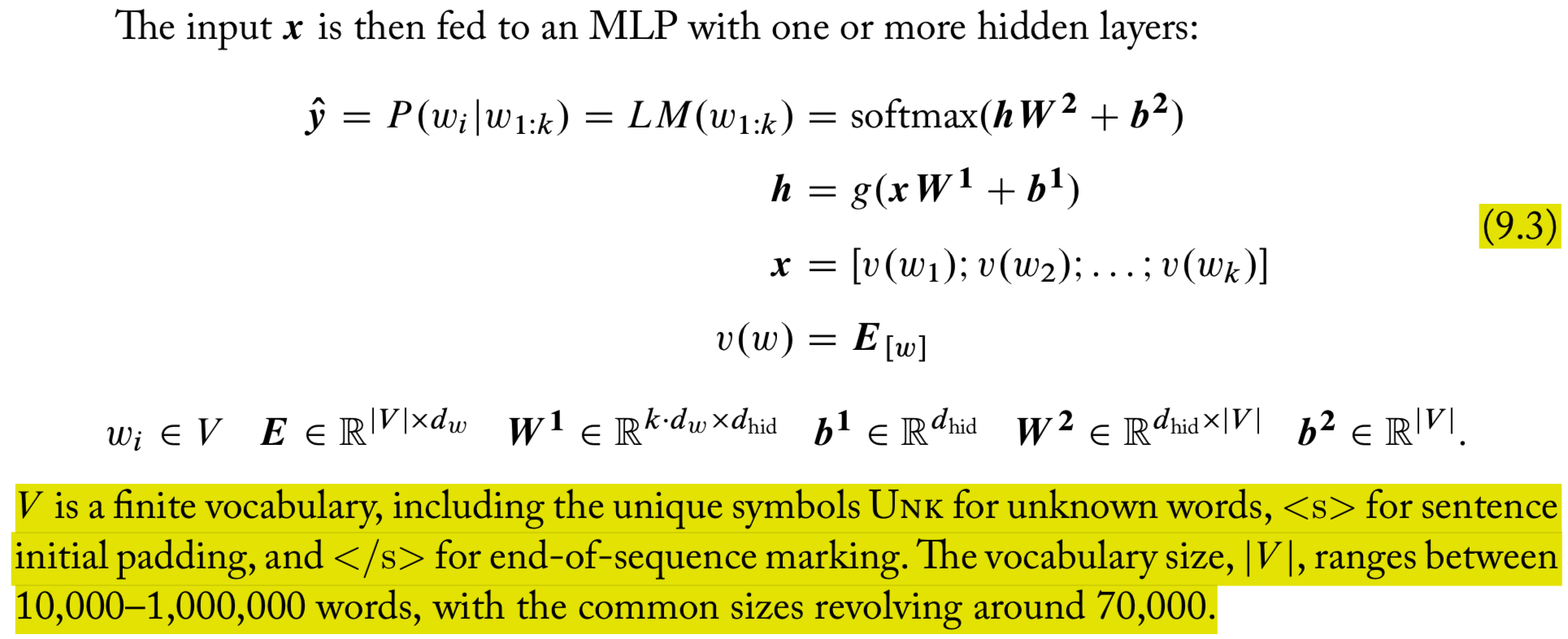
Neural language models
- Input to the neural network is a \(k\)gram of words \(w_{1:k}\), and the output is a probability distribution over the next word
Approximation of the softmax operation in cross entropy
Cross entropy loss works very well, but requires the use of a costly softmax operation which can be prohibitive for very large vocabularies
- This promotes the use of alternative losses and/or approximations
- Hierarchical softmax (using tree)
- Self-normalizing approaches, e.g., noise-contrastive estimation (NCE)
- Sampling approaches
NCE: replaces the cross-entropy objective with a collection of binary classification problems, requiring the evaluation of the assigned scores for \(k\) random words rather than the entire vocabulary
Using language models for generation
Predict a probability distribution over the first word conditioned on the start symbol, and draw a random word according to the predicted distribution
Then predict a probability distribution over the second word conditioned on the first
And so on, until predicting the end-of-sequence \(</s>\) symbol
Already with \(k=3\) this produces very passable text, and the quality improves with higher orders
Another option is to use beam search in order to find a sequence with a globally high probability
Ch10 Pre-trained Word Representations
Random initialization of word embedding models
The Word2Vec model initializes word vectors to uniformly sampled numbers in the range \(\left[-\frac{1}{2d}, \frac{1}{2d}\right]\)
Another option is xavier initialization, initializing with uniformly sampled numbers in the range \(\left[-\frac{\sqrt{6}}{\sqrt{d}}, \frac{\sqrt{6}}{\sqrt{d}}\right]\)
Unsupervised training of word embedding vectors
Key idea: one would like the embedding vectors of “similar” words to have similar vectors
Word similarity is from the distributional hypothesis: words are similar if they appear in similar contexts
The different methods all create supervised training instances in which the goal is to
- either predict the word from its context,
- or predict the context from the word
An important benefit of training word embedding on large amount of unannotated data: it provides vector representations for words that do not appear in the supervised training set
Word Simiarlity Matrices and SVD
Word-context matrices
Denote \(V_W\) the st of words and \(V_C\) the set of possible contexts
Assume that \(w_i\) is the \(i\)th word in the words vocabulary and \(c_j\) is the \(j\)th word in the context vocabulary
The matrix \(\mathbf{M}^f \in \mathbb{R}^{|V_W| \times |V_C|}\) is the word-context matrix, with \(f\) being an association measure of the strength between a word and a context \[ \mathbf{M}^f_{[i,j]} = f(w_i, c_j) \]
Similarity measures
- When words are represented as vectors, one can computing similarity by cosine similarity \[\begin{align*} \text{sim}_{\text{cos}} &= \frac{\mathbf{u} \cdot \mathbf{v}} {\|\mathbf{u}\|_2 \|\mathbf{v}\|_2}\\ &=\frac{\sum_i\mathbf{u}_{[i]} \cdot \mathbf{v}_{[i]}} {\sqrt{\sum_i(\mathbf{u}_{[i]})^2} \sqrt{\sum_i(\mathbf{v}_{[i]})^2}} \end{align*}\]
Word-context weighting and PMI
Denote by \(\#(w, c)\) the number of times word \(w\) occurred in the context \(c\) in the corpus \(D\), and let \(|D|\) be the corpus size
Pointwise mutual information (PMI) \[ \text{PMI}(w, c) = \log \frac{P(w, c)}{P(w) P(c)} = \log \frac{\#(w, c) |D|}{\#(w) \#(c)} \]
To resolve the \(\log 0\) issue for pairs \((w, c)\) never observed in the corpus, we can use the positive PMI (PPMI) \[ \text{PPMI}(w,c) = max\{\text{PMI}(w, c), 0\} \]
A deficiency of PMI: it tends to assign high value to rare events
Solution: it is advisable to apply a count threshold (to discount rare events) before using the PMI metric
Dimensionality reduction through matrix factorization
Potential obstacle of representing words as the explicit set of contexts: data sparsity, some entries in \(\mathbf{M}\) may be incorrect because we don’t have enough data points
Also, the explicit word vectors (row in \(\mathbf{M}\)) are of a very high dimension
Both issues can be alleviated by using dimension reduction techniques, e.g., singular value decomposition (SVD)
Mathematics of SVD
A \(m\times n\) matrix \(\mathbf{M}\) can be factorized into \[ \begin{array}{ccccc} \mathbf{M} & = & \mathbf{U} &\mathbf{D} & \mathbf{V}^T\\ m\times n & & m\times m & m\times n & n\times n \end{array} \]
- Matrix \(\mathbf{D}\) is diagonal. Matrices \(\mathbf{U}\) and \(\mathbf{V}\) are orthonormal, i.e., their rows are unit-length and orthogonal to each other
Dimension reduction under SVD: with a small value \(d\), \[ \begin{array}{ccccc} \mathbf{M}' & = & \tilde{\mathbf{U}} & \tilde{\mathbf{D}} & \tilde{\mathbf{V}}^T \\ m\times n & & m\times d & d\times d & d\times n \end{array} \]
- \(\mathbf{M}'\) is the best rank-\(d\) approximation of \(\mathbf{M}\) under the \(L_2\) loss
Use SVD to obtain word vectors
The low-dimensional rows of \[ \mathbf{W} = \tilde{\mathbf{U}} \tilde{\mathbf{D}} \] are low-rank approximations of the high-dimensional rows of the original matrix \(\mathbf{M}\)
- In the sense that computing the dot product between rows of \(\mathbf{W}\) is equivalent to computing dot product between the reconstructed matrix \(\mathbf{M}'\). \[ \mathbf{W}_{[i]} \cdot \mathbf{W}_{[j]} = \mathbf{M}'_{[i]} \cdot \mathbf{M}'_{[j]} \]
When using SVD for word similarity, the rows of \(\mathbf{M}\) correspond to words, the columns to contexts. Thus the rows of \(\mathbf{W}\) are low-dimensional word representations.
In practice, it is often better to not use \(\mathbf{W} = \tilde{\mathbf{U}} \tilde{\mathbf{D}}\), but instead to use the more balanced version \(\mathbf{W} = \tilde{\mathbf{U}} \sqrt{\tilde{\mathbf{D}}}\), or even directly using \(\mathbf{W} = \tilde{\mathbf{U}}\)
Collobert and Weston’s algorithm
Instead of computing a probability distribution over target words given a context, Collobert and Weston’s model only attempts to assign a score to each word, such that the correct word scores above the incorrect ones (p123)
Denote \(w\) the target word, \(c_{1:k}\) an ordered list of context items
Let \(v_w(w)\) and \(v_c(c)\) be embedding functions mapping word and context indices to \(d_{\text{emb}}\) dimensional vectors
Word2Vec Model
Word2Vec model: overview
- Word2Vec is a software package implementing
- two different context representations (CBOW and Skip-Gram) and
- two different optimization objectives (Negative-Sampling and Hierarchical Softmax)
- Here, we focus on the Negative-Sampling (NS) objective
Word2Vec model: negative sampling
Consider a set \(D\) of correct word-context pairs, and a set \(\bar{D}\) of incorrect word-context pairs
Goal: estimate the probability \(P(D=1 \mid w, c)\), which should be high (1) for pairs from \(D\) and low (0) for pairs from \(\bar{D}\)
The probability function: a sigmoid over the score \(s(w, c)\) \[ P(D=1 \mid w, c) = \frac{1}{1 + e^{-s(w, c)}} \]
The corpus-wide objective function is to maximize the log-likelihood of the data \(D \cup \bar{D}\) \[ \mathcal{L}(\Theta; D, \bar{D}) = \sum_{(w, c)\in D}\log P(D=1\mid w, c) + \sum_{(w, c)\in \bar{D}}\log P(D=0\mid w, c) \]
NS approximates the softmax function (normalizing term expensive to compute) with sigmoid functions
Word2Vec: NS, continued
The positive examples \(D\) are generated from a corpus
The negative samples \(\bar{D}\) can be generated as follows
For each good pair \((w, c)\in D\), sample \(k\) words \(w_{1:k}\) and add each of \((w_i, c)\) as a negative example to \(\bar{D}\). This results in \(\bar{D}\) being \(k\) times as large as \(D\). The number of negative samples \(k\) is a parameter of the algorithm
The negative words \(w\) can be sampled according to their corpus-based frequency. Actually in Word2Vec implementation, a smoothed version in which the counts are raised to the power of \(\frac{3}{4}\) before normalizing: \[ \frac{\#(w)^{0.75}}{\sum_{w'} \#(w')^{0.75}} \] This version gives more relative weights to less frequent words, and results in better word similarities in practice.
Word2Vec: CBOW
For a multi-word context \(c_{1:k}\), the CBOW variant of Word2Vec defines the context vector \(\mathbf{c}\) to be a sum of the embedding vectors of the context components \[ \mathbf{c} = \sum_{i=1}^k \mathbf{c}_i \]
The score of the word-context pair is simply defined as \[ s(w, c) = \mathbf{w} \cdot \mathbf{c} \]
Thus, the probability of a true pair is \[ P(D = 1\mid w, c_{1:k}) = \frac{1}{1 + e^{-(\mathbf{w} \cdot \mathbf{c}_1 + \mathbf{w} \cdot \mathbf{c}_2 + \cdots + \mathbf{w} \cdot \mathbf{c}_k)}} \]
The CBOW variant loses the order information between the context’s elements
In return, it allows the use of variable-length contexts
Word2Vec: Skip-Gram
For a \(k\)-element context \(c_{1:k}\), the skip-gram variant assumes that the elements \(c_i\) in the context are independent from each other, essentially treating them as \(k\) different contexts: \((w, c_1), (w, c_2), \ldots, (w, c_k)\)
The scoring function is the same as the CBOW version \[ s(w, c_i) = \mathbf{w} \cdot \mathbf{c_i} \]
The probability is a product of \(k\) terms \[ P(D = 1\mid w, c_{1:k}) = \prod_{i=1}^k P(D = 1\mid w, c_i) = \prod_{i=1}^k \frac{1}{1 + e^{-\mathbf{w} \cdot \mathbf{c}_i}} \]
While the independence assumption is strong, the skip-gram variant is very effective in practice
GloVe
- GloVe constructs an explicit word-context matrix, and trains the word and context vectors \(\mathbf{w}\) and \(\mathbf{c}\) attempting to satisfy \[ \mathbf{w} \cdot \mathbf{c} + \mathbf{b}_{[w]} + \mathbf{b}_{[c]} = \log \#(w, c), \quad \forall (w, c) \in D \] where \(\mathbf{b}_{[w]}\) and \(\mathbf{b}_{[c]}\) are word-specific and context-specific trained biases
Choice of Contexts
Choice of contexts: window approach
The most common is a sliding window approach, containing a sequence of \(2m+1\) words. The middle word is called the focus word and the \(m\) words to each side are the contexts
Effective window size: usually 2-5.
Larger windows tend to produce more topical similarities (e.g., “dog”, “bark”, and “leash” will be grouped together, as well as “walked”, “run”, and “walking”)
Smaller windows tend to produce more functional and syntactic similarities (e.g., “Poodle”, “Pitbull”, and “Rottweiler”, or “walking”, “running”, and “approaching”)
Many variants on the window approach are possible. One may
- lemmatize words before learning
- apply text normalization
- filter too short of too long sentences
- remove capitalization
Limitations of distributional methods
Black sheep: people are less likely to mention known information than they are to mention novel ones
- For example, when people talk of white sheep, they will likely refer to them as sheep, while for black sheep are are much more likely to retain the color information and say black sheep
Antonyms: words are opposite of each other (good vs bad, buy vs sell, hot vs cold) tend to appear in similar contexts
Ch11 Using Word Embeddings
Resources of Common Pre-Training Word Embeddings
Common pre-training word embeddings
Efficient implementation of Word2Vec
- GenSim python package: https://radimrehurek.com/gensim/
Efficient implementation of GloVe
Usages: Find Similarity, Word Analogies
Pre-trained word embedding usages
Calculate word similarity, e.g., using cosine similarity
Word clustering, e.g., using KMeans
Find similar words
With row-normalized embedding matrix, the cosine similarity between two words \(w_1\) and \(w_2\) is \[ \text{sim}_{\text{cos}}(w_1, w_2) = \mathbf{E}_{[w_1]} \cdot \mathbf{E}_{[w_2]} \]
We are often interested in the \(k\) most similar words to a given word \(w\). Let \(\mathbf{w} = \mathbf{E}_{[w]}\), then the similarity to all other words can be computed by the matrix-vector multiplication \[ \mathbf{s} = \mathbf{E} \mathbf{w} \]
More similarity measures
Similarity to a group of words: average similarity to the items in the group \[ \mathbf{s}_{[w]} = \text{sim}(w, w_{1:k}) = \mathbf{E} (\mathbf{w}_1 + \cdots + \mathbf{w}_k) / k \]
Short document similarity: consider two documents \(D_1 = w_1^1, \ldots, w_m^1\) and \(D_2 = w_1^2, \ldots, w_n^2\), \[\begin{align*} \text{sim}_{\text{doc}}(D_1, D_2) &= \sum_{i=1}^m \sum_{j=1}^n \text{cos}(\mathbf{w}_i^1, \mathbf{w}_j^2)\\ &= \left(\sum_{i=1}^m \mathbf{w}_i^1 \right) \cdot \left(\sum_{j=1}^n \mathbf{w}_j^2 \right) \end{align*}\]
Word analogies
One can perform “algebra” on the word vectors and get meaningful results
- For example, \[ \mathbf{w}_{\text{king}} - \mathbf{w}_{\text{man}} + \mathbf{w}_{\text{woman}} \approx \mathbf{w}_{\text{queen}} \]
Analogy solving task: to answer analogy questions of the form \[ man : woman \rightarrow king:? \]
Solve the analogy question by maximization \[\begin{align*} \text{analogy}(m:w \rightarrow k:?) & = \arg\max_{v \in V\backslash \{m, w, k\}} \text{cos}(\mathbf{v}, \mathbf{k} - \mathbf{m} + \mathbf{w}) \end{align*}\]
Practicalities and pitfalls
While off-the-shelf, pre-trained word embeddings can be downloaded and used, it is advised to not just blindly download word embeddings and treat them as a black box
Be aware of choices such as the source of the training corpus
- Larger training corpus is not always better. A smaller but cleaner, or smaller but more domain-focused corpus are often more effective
When using off-the-shelf embedding vectors, it is better to use the same tokenization and text normalization schemes that were used when deriving the corpus
References
- Goldberg, Yoav. (2017). Neural Network Methods for Natural Language Processing, Morgan & Claypool