Piecewise linear basis: tent functions

The problem with polynomials

• A k$k$th order polynomial is f(x)=β0+k∑j=1βkxk$$f\left(x\right)={\beta }_0+\sum _{j=1}^k{\beta }_k{x}^k$$

• The polynomial oscillates wildly in places, in order to both interpolate the data and to have all derivatives wrt x$x$ continuous

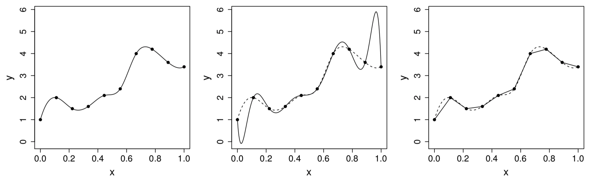
Figure 1: Left: the target function f(x)$f\left(x\right)$. Middle: polynomial interpolation. Right: piecewise linear interpolant

Visualization of tent function basis

• bj(x)$b_j\left(x\right)$ is zero everywhere, except over the interval between the knots immediately to either side of x∗j$x_j^{\ast }$

• bj(x)$b_j\left(x\right)$ increases linear from 0$0$ at x∗j−1$x_{j-1}^{\ast }$ to 1 at x∗j$x_j^{\ast }$, and then decreases linearly to 0$0$ at x∗j+1$x_{j+1}^{\ast }$

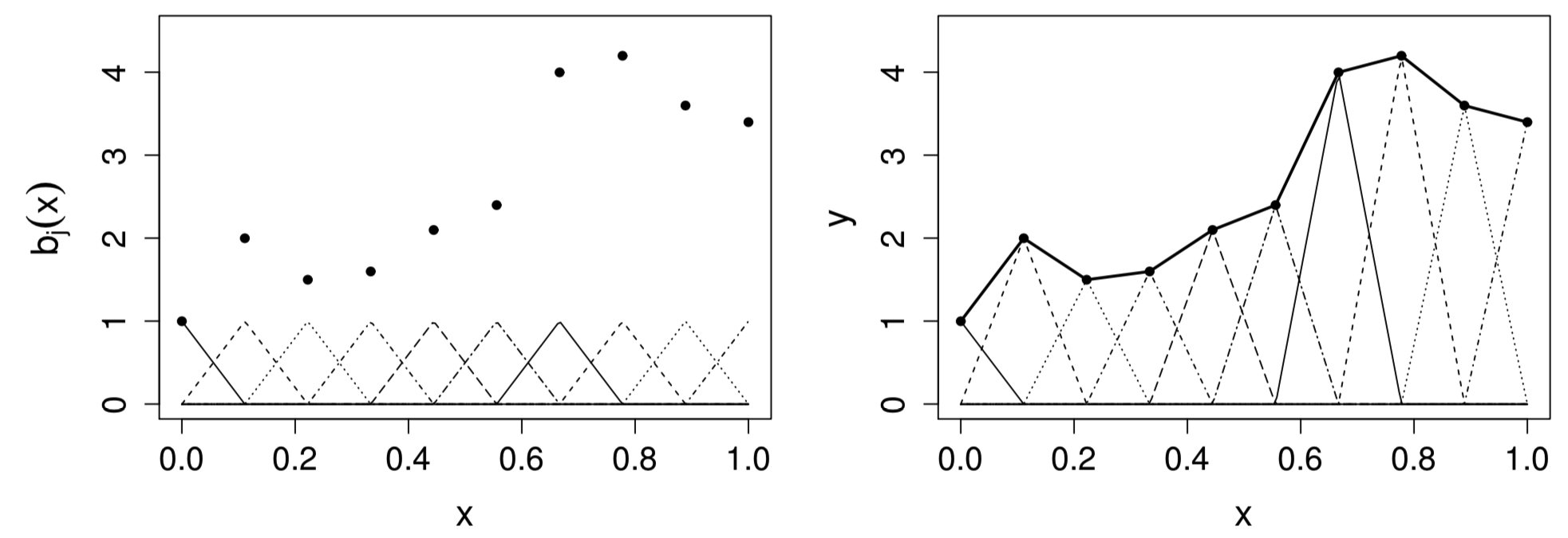
Figure 2: Left: tent function basis, for interpolating the data shown as black dots. Right: the basis functiosn are each multiplied by a coefficient, before being summed

Penalty to control wiggliness

A simple additive model with two univariate functions

• Let’s consider a simple additive model yi=α+f1(xi)+f2(vi)+ϵi,ϵiiid∼N(0,σ2)$$y_i=\alpha +f_1\left(x_i\right)+f_2\left(v_i\right)+{ϵ}_i,{ϵ}_i\stackrel{\text{iid}}{\sim }\text{N}(0,{\sigma }^2)$$

• The assumption of additive effects is a fairly strong one

• The model now has an identifiability problem: f1$f_1$ and f2$f_2$ are each only estimable to within an additive constant

  • Due to the identifiability issue, we need to use penalized regression splines

Piecewise linear regression representation

• Basis representation of f1()$f_1\left(\right)$ and f2()$f_2\left(\right)$ f1(x)=k1∑j=1bj(x)δjf2(v)=k2∑j=1Bj(v)γj$$\begin{array}{c}{f}_1\left(x\right)=\sum _{j=1}^{k_1}{b}_j\left(x\right){\delta }_j\\ f_2\left(v\right)=\sum _{j=1}^{k_2}{B}_j\left(v\right){\gamma }_j\end{array}$$

  • The basis functions bj()$b_j\left(\right)$ and Bj()$B_j\left(\right)$ are tent functions, with evenly spaced knots x∗j$x_j^{\ast }$ and v∗j$v_j^{\ast }$, respectively

• Matrix representations f1=[f1(x1),…,f1(xn)]T=X1δ,[X1]i,j=bj(xi)f2=[f2(v1),…,f2(vn)]T=X2γ,[X2]i,j=Bj(xi)$$\begin{array}{cc}{f}_1& =\left[f_1\right(x_1),\dots ,f_1(x_n){]}^T=X_1\delta ,[X_1{]}_{i,j}=b_j\left(x_i\right)\\ f_2& =\left[f_2\right(v_1),\dots ,f_2(v_n){]}^T=X_2\gamma ,[X_2{]}_{i,j}=B_j\left(x_i\right)\end{array}$$

Sum-to-zero constrains to resolve identifiability issues

• We assume n∑i=1f1(xi)=0⟺1Tf1=0$$\sum _{i=1}^n{f}_1\left(x_i\right)=0⟺1^T{f}_1=0$$ This is equivalent to 1TX1δ=0$1^T{X}_1\delta =0$ for all δ$\delta$, which implies 1TX1=0$1^T{X}_1=0$

• To achieve this condition, we can center the column of X1$X_1$ ˜X1=X1−1 1TX1n,˜f1=˜X1δ$${\tilde{X}}_1=X_1-1\frac{1^T{X}_1}{n},{\tilde{f}}_1={\tilde{X}}_1\delta$$

• Column centering reduces the rank of ˜X1${\tilde{X}}_1$ to k1−1$k_1-1$, so that only k1−1$k_1-1$ elements of the k1$k_1$ vector δ$\delta$ can be uniquely estimated

• A simple identifiability constraint:
  • Set a single element of δ$\delta$ to zero
  • And delete the corresponding column of ˜X1${\tilde{X}}_1$ and D$D$

• For notation simplicity, in what follows the tildes will be dropped, and we assume that the Xj$X_j$, Dj$D_j$ are the constrained versions

Penalized piecewise regression additive model

• We rewrite the penalized regression as y=Xβ+ϵ$$y=X\beta +ϵ$$ where X=(1,X1,X2)$X=(1,X_1,X_2)$ and βT=(α,δT,γT)${\beta }^T=(\alpha ,{\delta }^T,{\gamma }^T)$

• Wiggliness penalties δTDT1D1δ=δTˉS1δ=βTS1β,S1=[0000ˉS10000]γTDT2D2γ=γTˉS2γ=βTS2β,$$\begin{array}{cc}{\delta }^T{D}_1^T{D}_1\delta & ={\delta }^T{\overline{S}}_1\delta ={\beta }^T{S}_1\beta ,S_1=\left[\begin{array}{ccc}0& 0& 0\\ 0& {\overline{S}}_1& 0\\ 0& 0& 0\end{array}\right]\\ {\gamma }^T{D}_2^T{D}_2\gamma & ={\gamma }^T{\overline{S}}_2\gamma ={\beta }^T{S}_2\beta ,\end{array}$$

Fitting additive models by penalized least squares

• Penalized least squares objective function ‖y−Xβ‖2+λ1βTS1β+λ2βTS2β$$\parallel y-X\beta {\parallel }^2+{\lambda }_1{\beta }^T{S}_1\beta +{\lambda }_2{\beta }^T{S}_2\beta$$

• Coefficient estimator ˆβ=(XTX+λ1S1+λ2S2)−1XTy$$\hat{\beta }={(X^{T}X+{\lambda }_1{S}_1+{\lambda }_2{S}_2)}^{-1}{X}^{T}y$$

• Hat matrix A=X(XTX+λ1S1+λ2S2)−1XT$$A=X{(X^{T}X+{\lambda }_1{S}_1+{\lambda }_2{S}_2)}^{-1}{X}^T$$

• Conditional posterior distribution β∣y∼N(ˆβ,ˆVβ),ˆVβ=(XTX+λ1S1+λ2S2)−1ˆσ2$$\beta \mid y\sim \text{N}(\hat{\beta },{\hat{V}}_{\beta }),{\hat{V}}_{\beta }={(X^{T}X+{\lambda }_1{S}_1+{\lambda }_2{S}_2)}^{-1}{\hat{\sigma }}^2$$

Choosing two smoothing parameters

• Since we now have two smoothing parameters λ1,λ2${\lambda }_1,{\lambda }_2$, grid searching for the GCV optimal values starts to become inefficient

• Instead, R function optim can be used to minimize the GCV score

• We can use log smoothing parameters for optimization to ensure that estimated smoothing parameters are non-negative

Generalized additive models

• Generalized additive models (GAMs): additive models +$+$ GLM g(μi)=α+f1(xi)+f2(vi)+ϵi$$g\left({\mu }_i\right)=\alpha +f_1\left(x_i\right)+f_2\left(v_i\right)+{ϵ}_i$$

• Penalized iterative least squares (PIRLS) algorithm: iterate the following steps to convergence

1. Given the current ˆη$\hat{\eta }$ and ˆμ$\hat{\mu }$, compute wi=1V(ˆμi)g′(ˆμi)2,zi=g′(ˆμi)(yi−ˆμi)+ˆηi

2. Let W=diag(wi), we obtain the new ˆβ by minimizing ‖√Wz−√WXβ‖2+λ1βTS1β+λ2βTS2β

Introducing package mgcv

• Main function: gam(), very much like the glm() function

• Smooth terms: s() for univariate functions and te() for tensors

• A gamma regression example log(E[\tt Volumei])=f1(\tt Heighti)+f2(\tt Girthi),\tt Volumei∼Gamma

library(mgcv) ## load the package data(trees)
ct1 <- gam(Volume ~ s(Height) + s(Girth),
           family=Gamma(link=log),data=trees)

• By default, the degree of smoothness of the fj is estimated by GCV

summary(ct1)

## 
## Family: Gamma 
## Link function: log 
## 
## Formula:
## Volume ~ s(Height) + s(Girth)
## 
## Parametric coefficients:
##             Estimate Std. Error t value Pr(>|t|)    
## (Intercept)  3.27570    0.01492   219.6   <2e-16 ***
## ---
## Signif. codes:  0 '***' 0.001 '**' 0.01 '*' 0.05 '.' 0.1 ' ' 1
## 
## Approximate significance of smooth terms:
##             edf Ref.df      F  p-value    
## s(Height) 1.000  1.000  31.32 7.07e-06 ***
## s(Girth)  2.422  3.044 219.28  < 2e-16 ***
## ---
## Signif. codes:  0 '***' 0.001 '**' 0.01 '*' 0.05 '.' 0.1 ' ' 1
## 
## R-sq.(adj) =  0.973   Deviance explained = 97.8%
## GCV = 0.0080824  Scale est. = 0.006899  n = 31

Parital residuals plots

• Pearson residuals added to the estimated smooth terms ˆϵpartial1i=f1(\tt Heighti)+ˆϵpi

par(mfrow = c(1, 2))
plot(ct1,residuals=TRUE)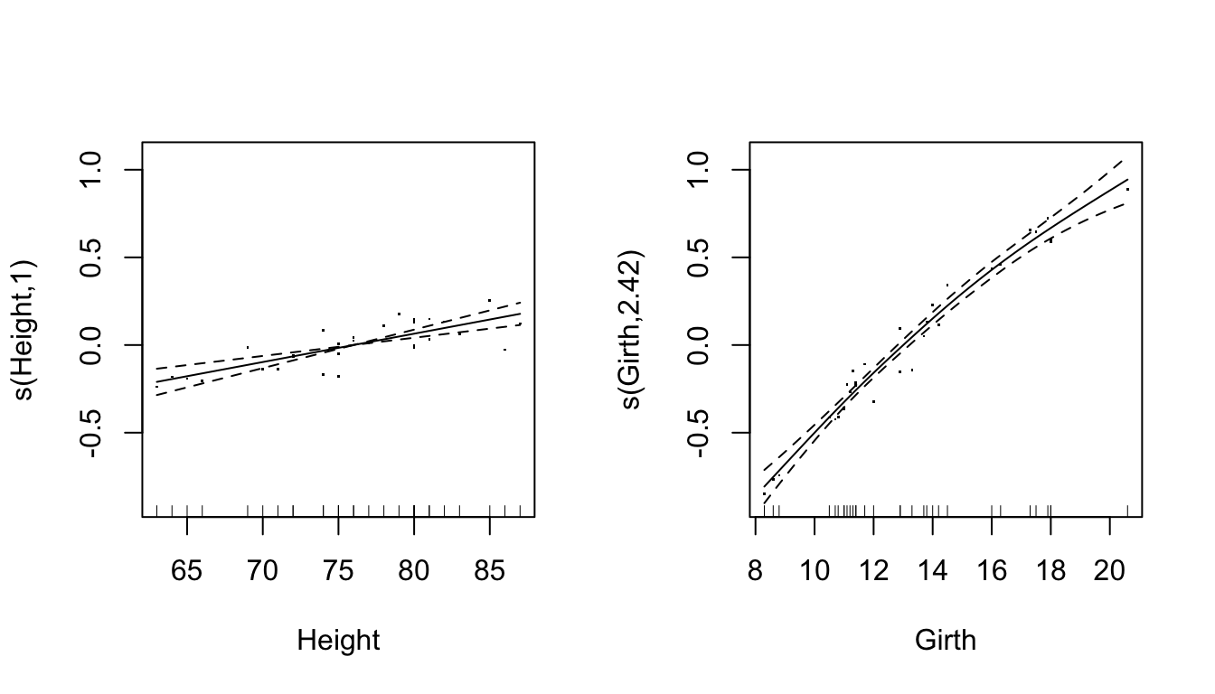

* The number in the y-axis label: effective degrees of freedom

Finer control of gam(): choice of basis functions

• Default: thin plat regression splines

  • It has some appealing properties, but can be somewhat computationally costly for large dataset

• We can select penalized cubic regression spline by using

s(..., bs = "cr")

• We can change the dimension k of the basis

  • The actual effective degrees of freedom for each term is usually estimated from the data by GCV or another smoothness selection criterion
  • The upper bound on this estimate is k−1, minus one due to identifiability constraint on each smooth term

s(..., bs = "cr", k = 20)

Finer control of gam(): the gamma parameter

• GCV is known to have some tendency to overfitting

• Inside the gam() function, the argument gamma can increase the amount of smoothing

  • The default value for gamma is 1
  • We can use a higher value to avoid overfitting, gamma = 1.5, without compromising model fit

References

• Wood, Simon N. (2017), Generalized Additive Models: An Introduction with R. Chapman and Hall/CRC