CNN overview for NLP

• CBOW assigns the following two sentences the same representations

  • “it was not good, it was actually quite bad”
  • “it was not bad, it was actually quite good”

• Looking at ngrams is much more informative than looking at a bag-of-words

• This chapter introduces the convolution-and-pooling (also called convolutional neural networks, or CNNs), which is tailored to this modeling problem

Benefits of CNN for NLP

• CNNs will identify ngrams that are predictive for the task at hand, without the need to pre-specify an embedding vector for each possible ngram

• CNNs also allows to share predictive behavior between ngrams that share similar components, even if the exact ngrams was never seen at test time

• Example paper: link

Convolution

• The main idea behind a convolution and pooling architecture of language tasks is to apply a non-linear (learned) function over each instantiation of a \(k\)-word sliding window over the sentence

• This function (also called “filter”) transforms a window of \(k\) words into a scalar value

  • Intuitively, when the sliding window of size \(k\) is run over a sequence, the filter function learns to identify informative \(k\)grams

• Several such filters can be applied, resulting in \(\ell\) dimensional vector (each dimension corresponding to one filter) that captures important properties of the words in the window

Pooling

• Then a “pooling” operation is used to combine the vectors resulting from the different windows into a single \(\ell\)-dimensional vector, by taking the max or the average value observed in each of the \(\ell\) dimensions over the different windows

  • The intention is to focus on the most important “features” in the sentence, regardless of their location

• The resulting \(\ell\)-dimensional vector is then fed further into a network that is used for prediction

1D convolutions over text

• A filter is a dot-product with a weight vector parameter \(\mathbf{u}\), which is often followed by nonlinear activation function

• Define the operation \(\oplus(\mathbf{w}_{i:i+k-1})\) to be the concatenation of the vectors \(\mathbf{w}_i, \ldots, \mathbf{w}_{i+k-1}\). The concatenated vector of the \(i\)th window is then \[ \mathbf{x}_i = \oplus(\mathbf{w}_{i:i+k-1}) = [\mathbf{w}_i; \mathbf{w}_{i+1}; \ldots; \mathbf{w}_{i+k-1}] \in \mathbb{R}^{k \cdot d_{\text{emb}}} \]

• Apply the filter to each window-vector, resulting scalar value \(p_i\): \[\begin{align*} &p_i = g(\mathbf{x}_i \cdot \mathbf{u})\\ &p_i \in \mathbb{R},\quad \mathbf{x}_i \in \mathbb{R}^{k \cdot d_{\text{emb}}}, \quad \mathbf{u} \in \mathbb{R}^{k \cdot d_{\text{emb}}} \end{align*}\]

Joint formulation of 1D convolutions

• It is customary to use \(\ell\) different filters \(\mathbf{u}_1, \ldots, \mathbf{u}_{\ell}\), which can be arranged into a matrix \(\mathbf{U}\), and a bias vector \(\mathbf{b}\) is often added

\[\begin{align*} &\mathbf{p}_i = g(\mathbf{x}_i \cdot \mathbf{U} + \mathbf{b})\\ &\mathbf{p}_i \in \mathbb{R}^{\ell},\quad \mathbf{x}_i \in \mathbb{R}^{k \cdot d_{\text{emb}}}, \quad \mathbf{U} \in \mathbb{R}^{k \cdot d_{\text{emb}} \times \ell}, \quad \mathbf{b} \in \mathbb{R}^{\ell} \end{align*}\]

• Ideally, each dimension captures a different kind of indicative information

• The main idea behind the convolution layer: to apply the same parameterized function over all \(k\)grams in the sequence. This creates a sequence of \(m\) vectors, each representing a particular \(k\)gram in the sequence

Narrow vs wide convolutions

• For a sentence of length \(n\) with a window of size \(k\)

• Narrow convolutions: there are \(n-k+1\) positions to start the sequence, and we get \(n-k+1\) vectors \(\mathbf{p}_{1:n-k+1}\)

• Wide convolutions: an alternative is to pad the sentence with \(k-1\) padding-words to each side, resulting in \(n+k+1\) vectors \(\mathbf{p}_{1:n+k+1}\)

• We use \(m\) to denote the number of resulting vectors

Vector pooling

• Applying the convolution over the text results in \(m\) vectors \(\mathbf{p}_{1:m}\), each \(\mathbf{p}_i \in \mathbb{R}^{\ell}\)

• These vectors are then combined (pooled) into a single vector \(\mathbf{c}\in \mathbb{R}^{\ell}\) representing the entire sequence

• During training, the vector \(\mathbf{c}\) is fed into downstream network layers (e.g., an MLP), culminating in an output layer which is used for prediction

Different pooling methods

• Max pooling: the most common, taking the maximum value across each dimension \(j = 1, \ldots, \ell\) \[ \mathbf{c}_{[j]} = \max_{1\leq i \leq m} \mathbf{p}_{i,[j]} \]

  • The effect of the max-pooling operation is to get the most salient information across window positions

• Average pooling \[ \mathbf{c} = \frac{1}{m}\sum_{i=1}^m \mathbf{p}_i \]

• \(K\)-max pooling: the top \(k\) values in each dimension are retained instead of only the best one, while preserving the order in which they appeared in the text

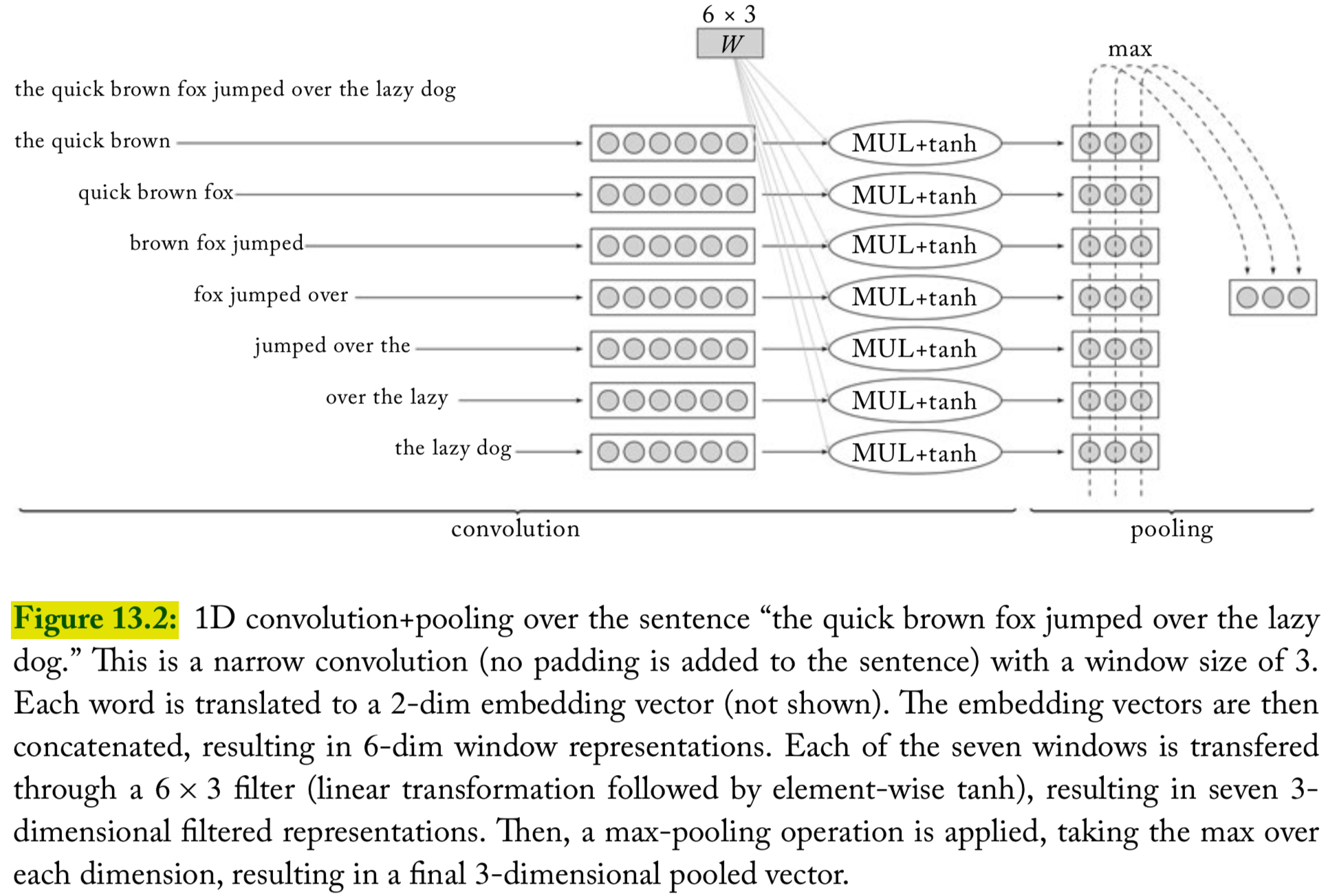
An illustration of convolution and pooling

Variations

• Rather than a single convolutional layer, several convolutional layers may be applied in parallel

• For example, we may have four different convolutional layers, each with a different window size in the range 2-5, capturing \(k\)gram sequences of varying lengths

Hierarchical convolutions

• The 1D convolution approach described so far can the thought of as a ngram detector: a convolution layer with a window of size \(k\) is learning to identify indicative \(k\)-gram in the input

\[ \mathbf{p}_{1:m} = \text{CONV}^k_{\mathbf{U}, \mathbf{b}}(\mathbf{w}_{1:n}) \]

• We can extend this into a hierarchy of convolutional layers with \(r\) layers that feed into each other \[\begin{align*} \mathbf{p}_{1:m_1}^1 & =\text{CONV}^{k_1}_{\mathbf{U}^1,\mathbf{b}^1}(\mathbf{w}_{1:n})\\ \mathbf{p}_{1:m_2}^2 & =\text{CONV}^{k_2}_{\mathbf{U}^2,\mathbf{b}^2}(\mathbf{p}_{1:m_1}^1)\\ &\cdots\\ \mathbf{p}_{1:m_r}^r & =\text{CONV}^{k_r}_{\mathbf{U}^r,\mathbf{b}^r}(\mathbf{p}_{1:m_{r-1}}^{r-1}) \end{align*}\]

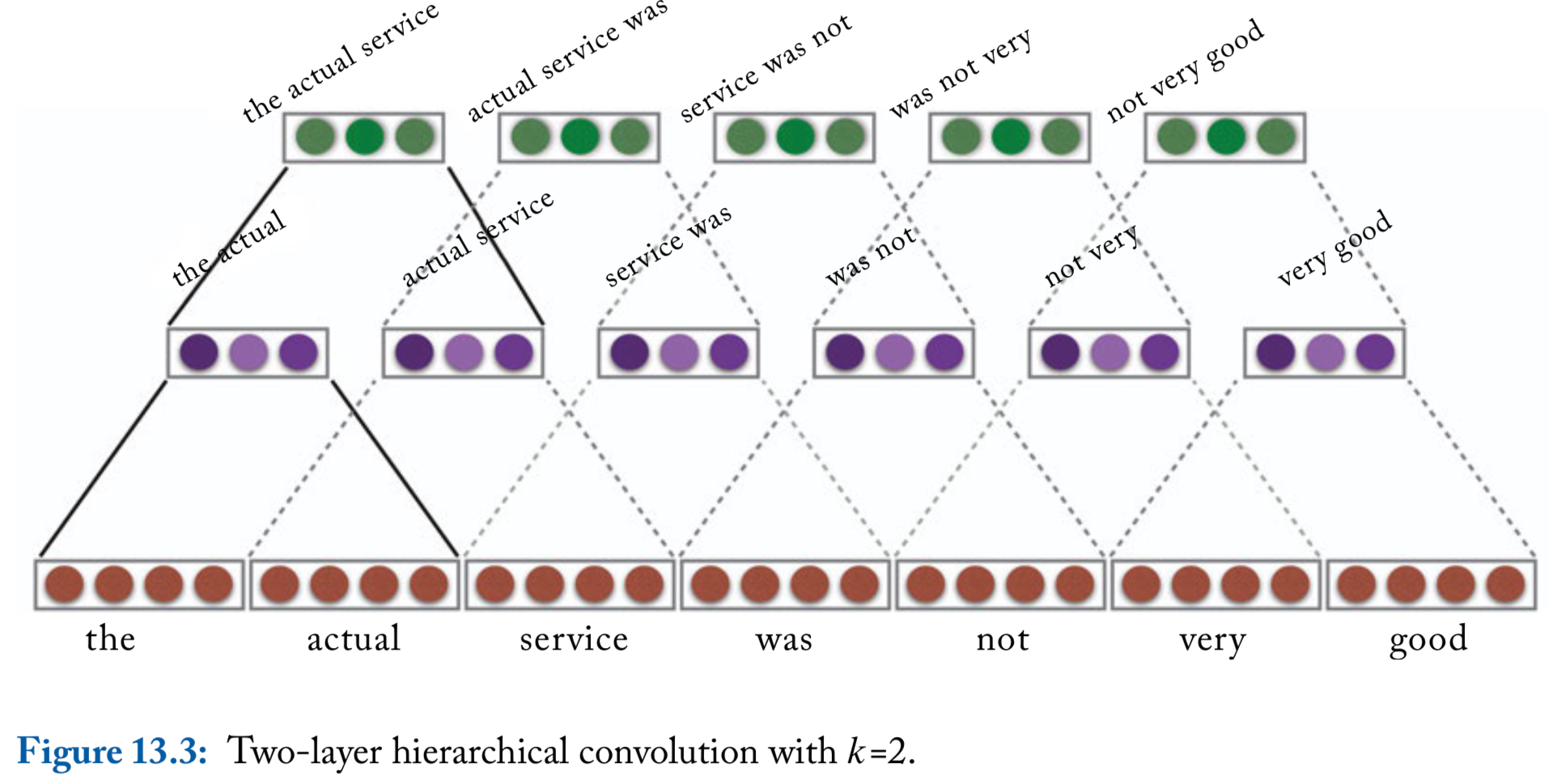
Hierarchical convolutions, continued

• For \(r\) layers with a window of size \(k\), each vector \(\mathbf{p}_i^r\) will be sensitive to a window of \(r(k-1)+1\) words

• Moreover, the vector \(\mathbf{p}_i^r\) can be sensitive to gappy-ngrams of \(k+r-1\) works, potentially capturing patterns such as “not ___ good” or “obvious ___ predictable ___ plot”, where ___ stands for a short sequence of words

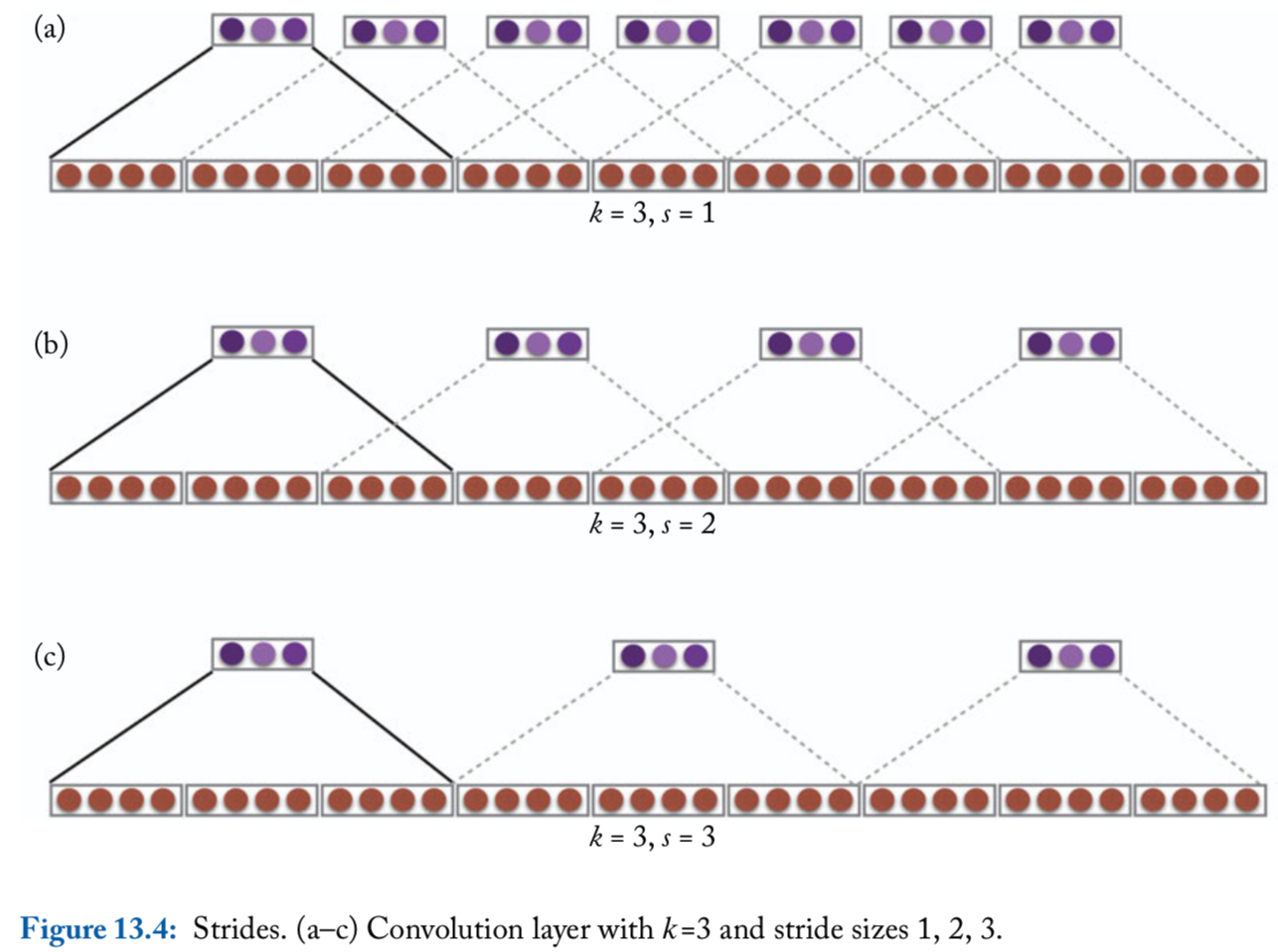
Strides

• So far, the convolution operation is applied to each \(k\)-word window in the sequence, i.e., windows starting at indices \(1, 2, 3, \ldots\). This is said to have a stride of size \(1\)

• Larger strides are also possible. For example, with a stride of size \(2\), the convolution operation will be applied to windows starting at indices \(1, 3, 5, \ldots\)

• Convolution with window size \(k\) and stride size \(s\): \[\begin{align*} \mathbf{p}_{1:m} &= \text{CONV}^{k,s}_{\mathbf{U}, \mathbf{b}}(\mathbf{w}_{1:n})\\ \mathbf{p}_i &= g\left(\oplus \left( \mathbf{w}_{1+(i-1)s : (s+k)i} \right) \cdot \mathbf{U} + \mathbf{b} \right) \end{align*}\]

An illustration of stride size

References

• Goldberg, Yoav. (2017). Neural Network Methods for Natural Language Processing, Morgan & Claypool