The RNN abstraction

• On a high level, the RNN is a function that

  • Takes as input an arbitrary length ordered sequence of \(n\) \(d_{\text{in}}\)-dimensional vectors \(\mathbf{x}_{1:n} = \mathbf{x}_1, \ldots, \mathbf{x}_n\), and
  • Returns as output a single \(d_{\text{out}}\) dimensional vector \(\mathbf{y}_n\)
  • The output vector \(\mathbf{y}_n\) is then used for further prediction \[\begin{align*} & \mathbf{y}_n = \text{RNN}(\mathbf{x}_{1:n})\\ & \mathbf{x}_i \in \mathbb{R}^{d_{\text{in}}}, \quad \mathbf{y}_n \in \mathbb{R}^{d_{\text{out}}} \end{align*}\]

• This implicitly defines an output vector \(\mathbf{y}_i\) for each prefix \(\mathbf{x}_{1:i}\). We denote by RNN\(^*\) the function returning this sequence \[\begin{align*} & \mathbf{y}_{1:n} = \text{RNN}^*(\mathbf{x}_{1:n})\\ & \mathbf{y}_i = \text{RNN}(\mathbf{x}_{1:i})\\ & \mathbf{x}_i \in \mathbb{R}^{d_{\text{in}}}, \quad \mathbf{y}_i \in \mathbb{R}^{d_{\text{out}}} \end{align*}\]

• The RNN function provides a framework for conditioning on the entire history \(\mathbf{x}_1, \ldots, \mathbf{x}_i\) without the Markov assumption

The R function and the O function

• The RNN is defined recursively, by means of a function \(R\) taking as the state vector \(\mathbf{s}_{i-1}\) and an input vector \(\mathbf{x}_i\) and returning a new state vector \(\mathbf{s}_i\)

• The state vector \(\mathbf{s}_i\) is then mapped to an output vector \(\mathbf{y}_i\) using a simple deterministic function \(O\) \[\begin{align*} \mathbf{s}_i & = R(\mathbf{s}_{i-1}, \mathbf{x}_i)\\ \mathbf{y}_i & = O(\mathbf{s}_i) \end{align*}\]

• The functions \(R\) and \(O\) are the same across the sequence positions, but the RNN keeps track of the states of computation through the state vector \(\mathbf{s}_i\) that is kept and being passed across invocations of \(R\)

An illustration of the RNN

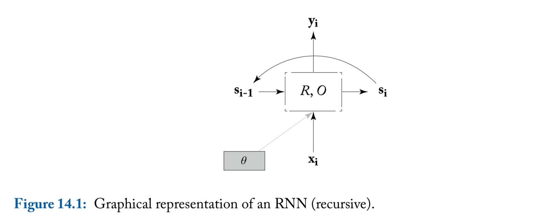
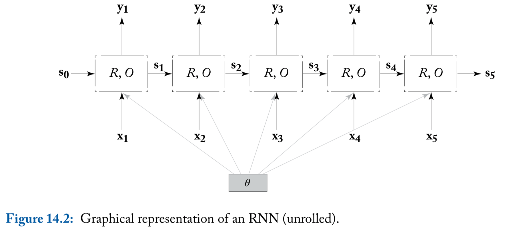
• We include here the parameters \(\theta\) in order to highlight the fact that the same parameters are shared across all time steps

An illustration of the RNN (unrolled)

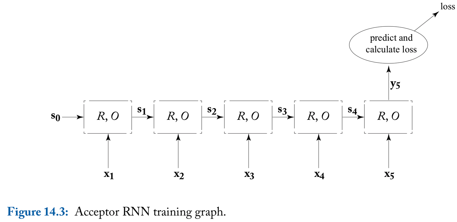
Common RNN usage patterns: acceptor

• Acceptor: based on the supervision signal only at the final output vector \(\mathbf{y}_n\)

  • Typically, the RNN’s output vector \(\mathbf{y}_n\) is fed into a fully connected layer or an MLP, which produce a prediction

Common RNN usage patterns: encoder

• Encoder: also only uses the final output vector \(\mathbf{y}_n\). Here \(\mathbf{y}_n\) is treated as an encoding of the information in the sequence, and is used as additional information together with other signals

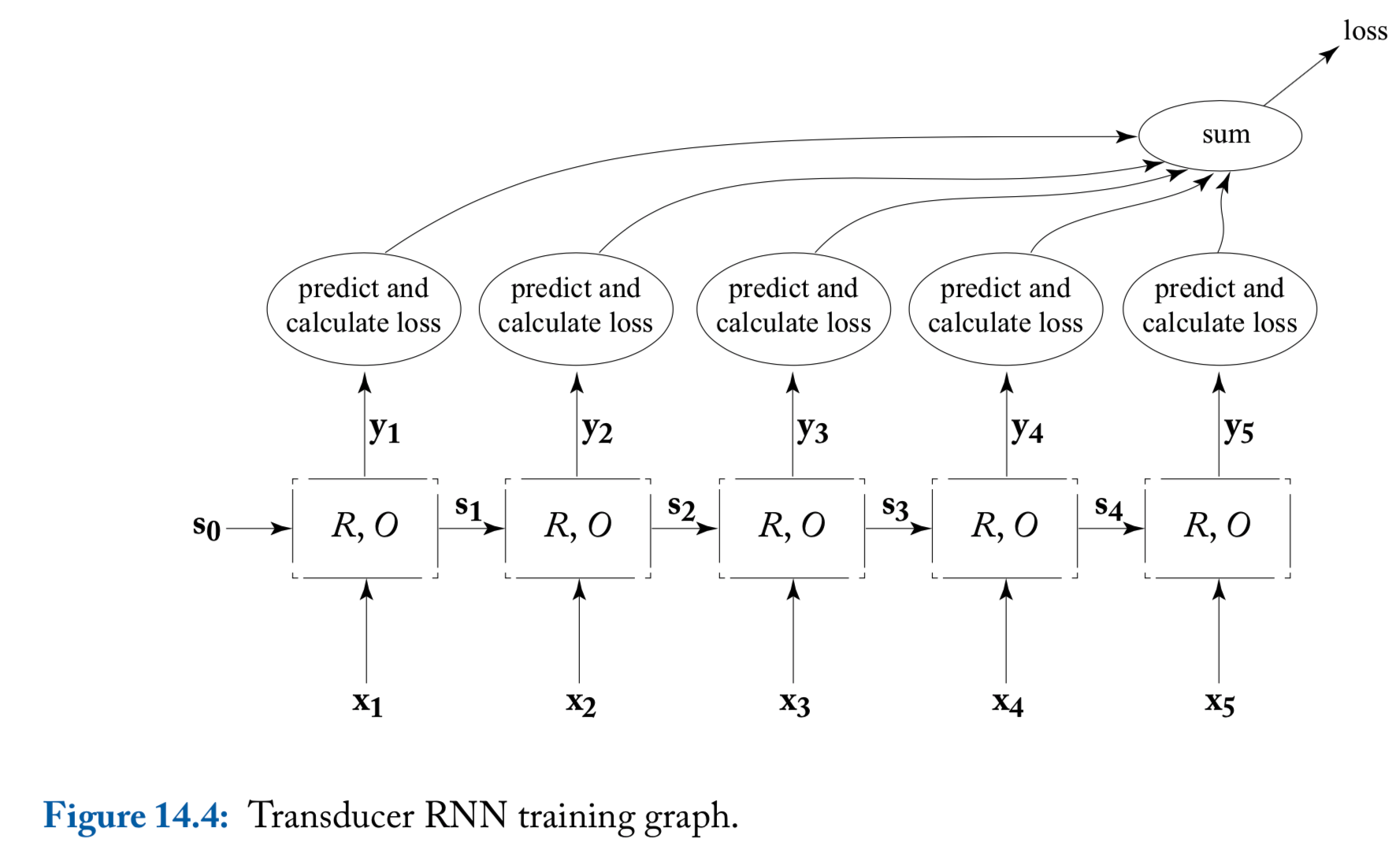
Common RNN usage patterns: transducer

• Transducer: The loss of unrolled sequence will be used

• A natural use case of the transduction is for language modeling, where the sequence of words \(\mathbf{x}_{1:i}\) is used to predict a distribution over the \((i+1)\)th word

• RNN based lanuage models are shown to provide vastly better perplxities than traditional language models

• Using RNNs as transducers allows us to relax the Markov assumption and condition on the entire prediction history

An illustration of transducer

Bidirectional RNNs (biRNN)

• A useful elaboration of an RNN is a biRNN

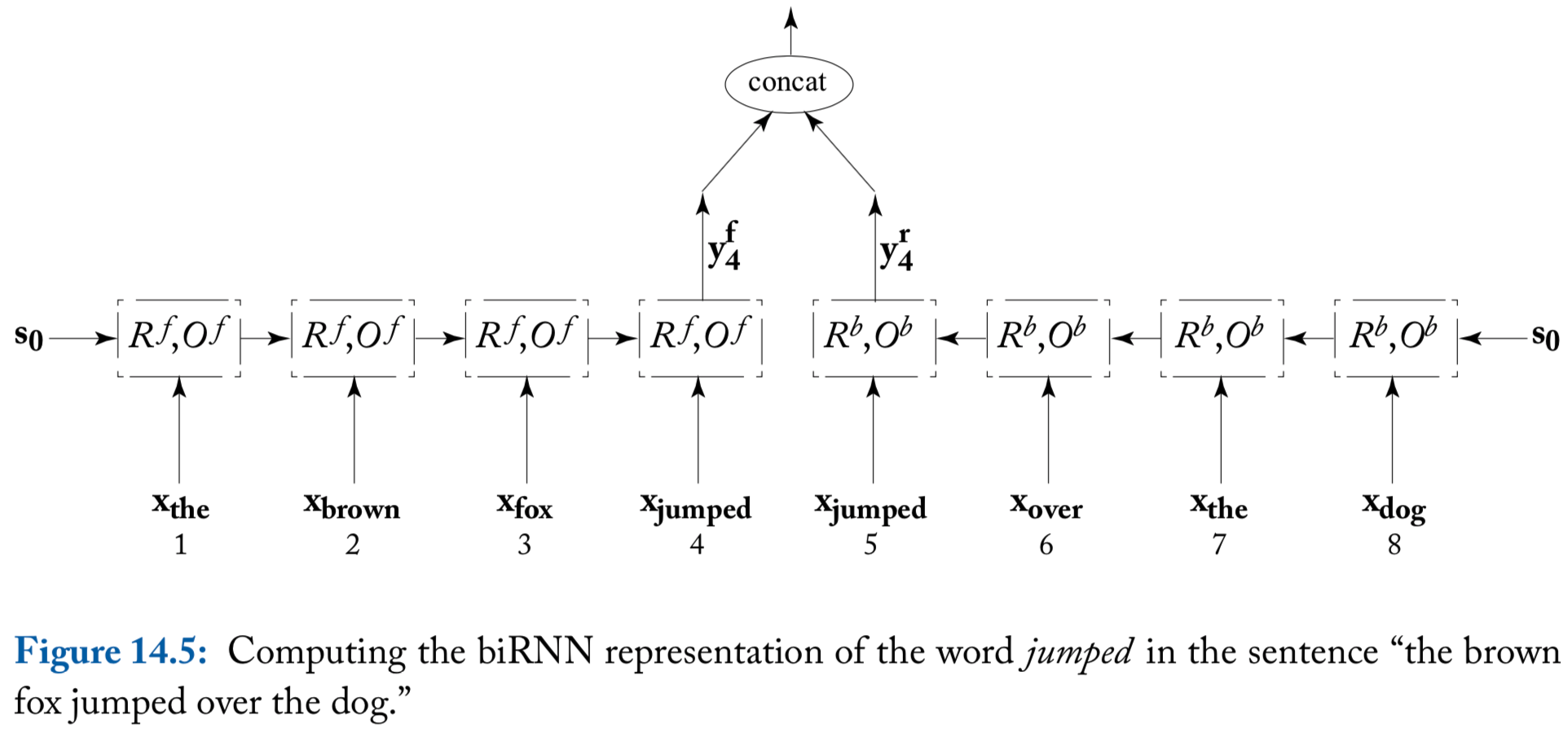
• Consider an input sequence \(\mathbf{x}_{1:n}\). The biRNN works by maintaining two separate states, \(\mathbf{s}_i^f\) and \(\mathbf{s}_i^b\) for each input position \(i\)

  • The forward state \(\mathbf{s}_i^f\) is based on \(\mathbf{x}_1, \mathbf{x}_2, \ldots, \mathbf{x}_i\)
  • The backward state \(\mathbf{s}_i^b\) is based on \(\mathbf{x}_n, \mathbf{x}_{n-1}, \ldots, \mathbf{x}_i\)

• The output at position \(i\) is based on the concatenation of the two output vectors \[ \mathbf{y}_i = \left[ \mathbf{y}_i^f; \mathbf{y}_i^b \right] = \left[ O^f(\mathbf{s}_i^f); O^b(\mathbf{s}_i^b) \right] \]

• Thus, we define biRNN as \[ \text{biRNN}(\mathbf{x}_{1:n}, i) = \mathbf{y}_i = \left[ \text{RNN}^f(\mathbf{x}_{1:i}), \text{RNN}^b(\mathbf{x}_{n:i}) \right] \]

An illustration of biRNN

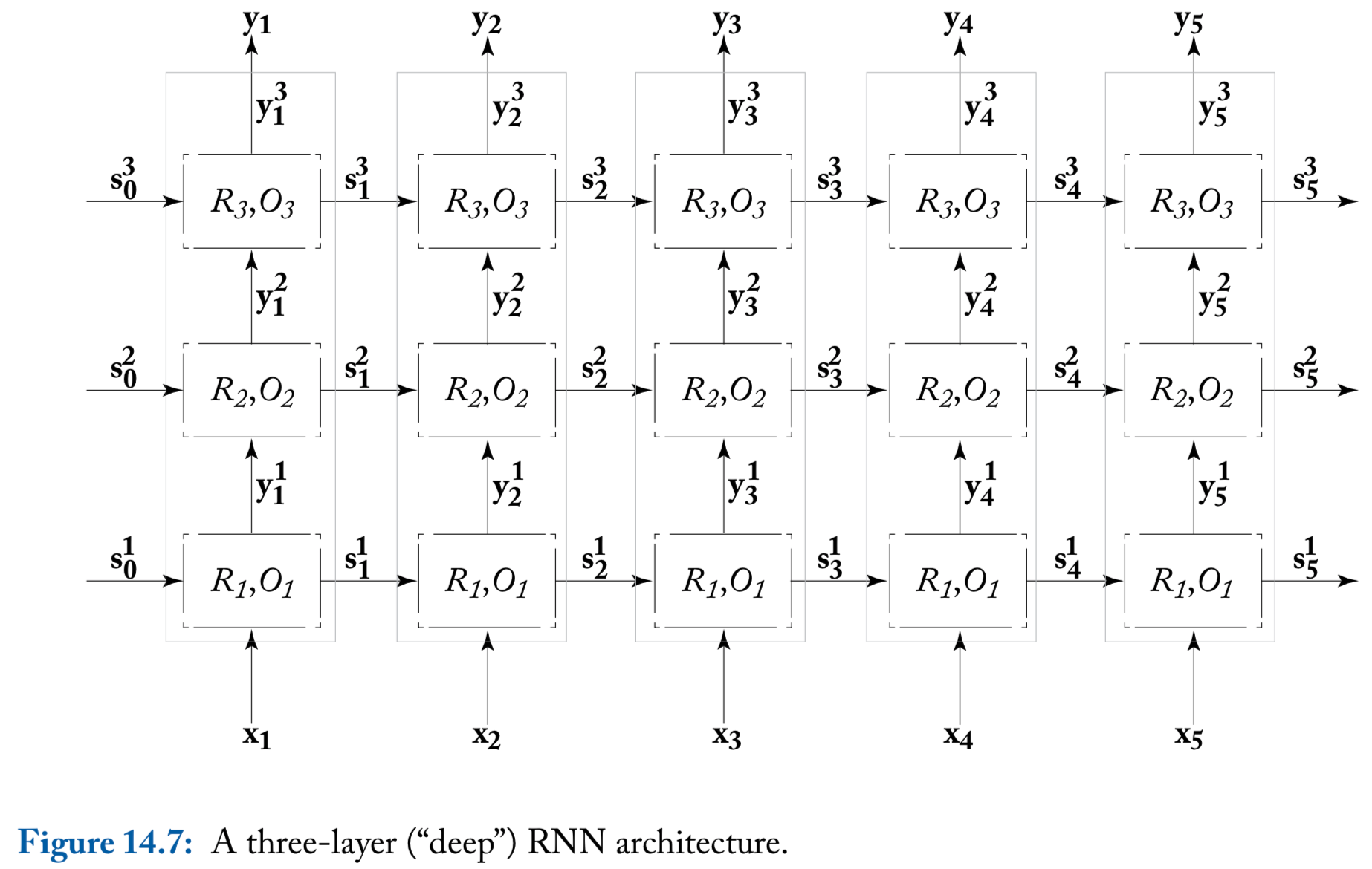
Deep (multi-layer stacked) RNNs

• The input for the first RNN are \(\mathbf{x}_{1:n}\), while the input of the \(j\)th RNN (\(j \geq 2\)) are the outputs of the RNN below it, \(\mathbf{y}_{1:n}^{j-1}\)

• While it is not theoretically clear what is the additional power gained by the deeper architecture, it was observed empirically that deep RNNs work better than shallower ones on some tasks

• The author’s experience: using two or more layers indeed often improves over using a single one

A note on reading the literature

• Unfortunately, it is often the case that inferring the exact model form from reading its description in a research paper can be quite challenging

• For example,
  • The inputs to the RNN can be either one-hot vectors or embedded representations
  • The input sequence can be padded with start-of-sequence and/or end-of-sequence symbols, or not

An illustration of deep RNN

Simple RNN (SRNN)

• The nonlinear function \(g\) is usually tanh or ReLU

• The output function \(O(\cdot)\) is the identify function \[\begin{align*} \mathbf{s}_i & = R_\text{SRNN}(\mathbf{x}_i, \mathbf{s}_{i-1}) = g\left( \mathbf{s}_{i-1} \mathbf{W}^s + \mathbf{x}_{i} \mathbf{W}^x + \mathbf{b} \right)\\ \mathbf{y}_i & = O_\text{SRNN}(\mathbf{s}_i) = \mathbf{s}_i \end{align*}\] \[ \mathbf{s}_i, \mathbf{y}_i \in \mathbb{R}^{d_s}, \quad \mathbf{x}_i \in \mathbb{R}^{d_x}, \quad \mathbf{W}^x \in \mathbb{R}^{d_x \times d_s}, \quad \mathbf{W}^s \in \mathbb{R}^{d_s \times d_s}, \quad \mathbf{b} \in \mathbb{R}^{d_s} \]

• SRNN is hard to train effectively because of the vanishing gradients problem

Gated architectures

• An apparent problem with SRNN is that the memory access is not controlled. At each step of the computation, the entire memory state is read, and the entire memory state is written

• We denote the hadamard-product operation (element-wise product) as \(\odot\)

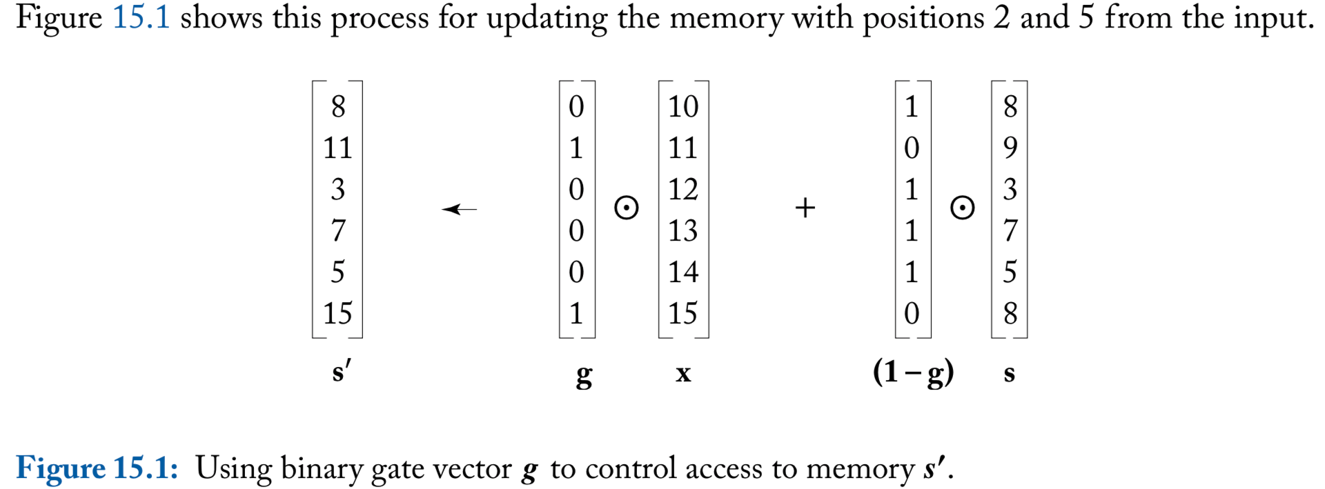
• To control memory access, consider a binary vector \(\mathbf{g} \in \{0, 1\}^{n}\)

• For a memory \(\mathbf{s} \in \mathbb{R}^d\) and an input \(\mathbf{x} \in \mathbb{R}^d\), the computation

\[ \mathbf{s}^{\prime} \longleftarrow \mathbf{g} \odot \mathbf{x} + (\mathbf{1} - \mathbf{g} ) \odot \mathbf{s} \] “reads” the entries in \(\mathbf{x}\) that correspond to the 1 values in \(\mathbf{g}\), and writes them to the new memory \(\mathbf{s}'\). Locations that weren’t read to are copied from the memory \(\mathbf{s}\) to the new memory \(\mathbf{s}'\) through the use of the gate \((1-\mathbf{g})\)

An illustration of binary gate

Differentiable gates

• The gates should not be static, but be controlled by the current memory state and the input, and their behavior should be learned

• Obstacle: learning in our framework entails being differentiable (because of the backpropagation algorithm), but the binary 0-1 values used in th e gates are not differentiable

• Solution: approximate the hard gating mechanism with a soft, but diffrentiable, gating mechanism

• To achieve these differentiable gates, we replace the requirement that \(\mathbf{g} \in \{0, 1\}^{n}\), and allow arbitrary real numbers \(\mathbf{g}' \in \mathbb{R}^{n}\). These are then passed through a sigmoid function \(\sigma(\mathbf{g}')\), which take values in the range \((0, 1)\)

LSTM

• Long Short-Term Memory (LSTM): explicitly splits the state vector \(\mathbf{s}_i\) into two halves, where one half is treated as “memory cells” \(\mathbf{c}_j\), and the hidden state component \(\mathbf{h}_j\)

\[ \mathbf{s}_j = \text{R}_{\text{LSTM}}(\mathbf{s}_{j-1}, \mathbf{x}_j) = \left[\mathbf{c}_j; \mathbf{h}_j \right] \]

• There are three gates, \(\mathbf{i}\)nput, \(\mathbf{f}\)orget, and \(\mathbf{o}\)utput \[\begin{align*} \mathbf{c}_j &= \mathbf{f} \odot \mathbf{c}_{j-1} + \mathbf{i} \odot \mathbf{z}\\ \mathbf{z} &= \text{tanh}\left(\mathbf{x}_j \mathbf{W}^{xz} + \mathbf{h}_{j-1} \mathbf{W}^{hz} \right)\\ \mathbf{h}_{j} &= \mathbf{o} \odot \text{tanh}(\mathbf{c}_j) \\ \mathbf{y}_j &= O_{\text{LSTM}}(\mathbf{s}_j) = \mathbf{h}_{j} \end{align*}\]

LSTM gates

• The gates are based on \(\mathbf{x}_j, \mathbf{h}_{j-1}\) and are passed through a sigmoid activation function \[\begin{align*} \mathbf{i} & = \sigma\left( \mathbf{x}_j \mathbf{W}^{xi} + \mathbf{h}_{j-1} \mathbf{W}^{hi} \right)\\ \mathbf{f} & = \sigma\left( \mathbf{x}_j \mathbf{W}^{xf} + \mathbf{h}_{j-1} \mathbf{W}^{hf} \right)\\ \mathbf{o} & = \sigma\left( \mathbf{x}_j \mathbf{W}^{xo} + \mathbf{h}_{j-1} \mathbf{W}^{ho} \right)\\ \end{align*}\]

• When training LSTM networks, it is strongly recommended to always initialize the bias term of the forget gate to be close to one

GRU

• Gated Recurrent Unit (GRU) is shown to perform comparably to the LSTM on several datasets

• GRU has substantially fewer gates that LSTM and doesn’t have a separate memory component \[\begin{align*} \mathbf{s}_j &= \text{R}_{\text{GRU}}(\mathbf{s}_{j-1}, \mathbf{x}_j) = \mathbf{(\mathbf{1} - \mathbf{z})} \odot \mathbf{s}_{j-1} + \mathbf{z} \odot \tilde{\mathbf{s}}_j\\ \tilde{\mathbf{s}}_j &= \text{tanh}\left( \mathbf{x}_j \mathbf{W}^{xs} + (\mathbf{r}\odot \mathbf{s}_{j-1}) \mathbf{W}^{sg}\right)\\ \mathbf{y}_j &= O_{\text{GRU}}(\mathbf{s}_j) = \mathbf{s}_{j} \end{align*}\]

• Gate \(\mathbf{r}\) controls access to the previous state \(\mathbf{s}_{j-1}\) in \(\tilde{\mathbf{s}}_j\)

• Gate \(\mathbf{z}\) controls the proportions of the interpolation between \(\mathbf{s}_{j-1}\) and \(\tilde{\mathbf{s}}_j\) when in the updated state \(\mathbf{s}_j\) \[\begin{align*} \mathbf{z} & = \sigma\left( \mathbf{x}_j \mathbf{W}^{xz} + \mathbf{s}_{j-1} \mathbf{W}^{sz} \right)\\ \mathbf{r} & = \sigma\left( \mathbf{x}_j \mathbf{W}^{xr} + \mathbf{s}_{j-1} \mathbf{W}^{sr} \right) \end{align*}\]

Acceptors

• The simplest use of RNN: read in an input sequence, and produce a binary of multi-class answer at the end

• The power of RNN is often not needed for many natural language classification tasks, because the word-order and sentence structure turn out to not be very important in many cases, and bag-of-words or bag-of-ngrams classifier often works just as well or even better than RNN acceptors

Sentiment classification: sentence level

• The sentence level sentiment classification is straightforward to model using an RNN acceptor:

  • Tokenization
  • RNN reads in the words of the sentence one at a time
  • The final RNN state is then fed into a MLP followed by a softmax-layer with two outputs
  • The network is trained with cross-entropy loss based on the gold sentiment labels \[\begin{align*} p(\text{label}=k \mid w_{1:n}) & = \hat{\mathbf{y}}_{[k]}\\ \hat{\mathbf{y}} &= \text{softmax}\left\{ \text{MLP}\left[\text{RNN}(x_{1:n}) \right] \right\}\\ \mathbf{x}_{1:n} &= \mathbf{E}_{[w_1]}, \ldots, \mathbf{E}_{[w_n]} \end{align*}\]

• biRNN: it is often helpful to extend the RNN model into the biRNN \[ \hat{\mathbf{y}} = \text{softmax}\left\{ \text{MLP}\left[\text{RNN}^f(x_{1:n}); \text{RNN}^b(x_{n:1}) \right] \right\} \]

Hierarchical biRNN

• For longer sentences, it can be useful to use a hierarchical architecture, in which the sentence is split into smaller spans based on punctuation

• Suppose a sentence \(w_{1:n}\) is split into \(m\) spans \(w_{1:\ell_1}^1, \ldots, w_{1:\ell_m}^m\), then the architecture is \[\begin{align*} p(\text{label}=k \mid w_{1:n}) & = \hat{\mathbf{y}}_{[k]}\\ \hat{\mathbf{y}} &= \text{softmax}\left\{ \text{MLP}\left[\text{RNN}(\mathbf{z}_{1:m})\right] \right\}\\ \mathbf{z}_i &= \left[\text{RNN}^f(\mathbf{x}_{1:\ell_i}^i), \text{RNN}^b(\mathbf{x}_{\ell_i:1}^i)\right] \\ \mathbf{x}_{1:\ell_i}^i &= \mathbf{E}_{[w_1^i]}, \ldots, \mathbf{E}_{[w_{\ell_i}^i]} \end{align*}\]

• Each of the \(m\) different spans may convey a different sentiment

• The higher-level acceptor reads the summary \(\mathbf{z}_{1:m}\) produced by the lower level encoder, and decides on the overall sentiment

Document level sentiment classification

• Document level sentiment classification and harder than sentence level classification

• A hierarchical architecture is useful:

  • Each sentence \(s_i\) is encoded using a gated RNN, producing a vector \(\mathbf{z}_i\)
  • The vectors \(\mathbf{z}_{1:n}\) are then fed into a second gated RNN, producing a vector \(\mathbf{h} = \text{RNN}(\mathbf{z}_{1:n})\)
  • \(\mathbf{h}\) is then used fro prediction \(\hat{\mathbf{y}} = \text{softmax}(\text{MLP}(\mathbf{h}))\)

• Keeping all intermediate vectors of the document-level RNN produces slightly higher results in some cases \[\begin{align*} \mathbf{h}_{1:n} &= \text{RNN}^*(\mathbf{z}_{1:n})\\ \hat{\mathbf{y}} &= \text{softmax}\left(\text{MLP}\left(\frac{1}{n}\sum_{i=1}^n\mathbf{h}_i\right)\right) \end{align*}\]

References

• Goldberg, Yoav. (2017). Neural Network Methods for Natural Language Processing, Morgan & Claypool