For the pdf slides, click here
Inverse Probability of Treatment Weighting
Motivating example
- Suppose there is a single confounder \(X\), with propensity scores \[ P(A=1\mid X=1) = 0.1, \quad P(A=1\mid X=0) = 0.8 \]

In propensity score matching, for subjects with \(X=1\), 1 out of 9 controls will be matched to the treated
Thus, 1 person in the treated group counts the same as 9 people from the control group
So rather than matching, we could use all data, but down-weight each control subject to be just 1/9 of the treated subject
Inverse probability of treatment weighting (IPTW)
IPTW weights: inverse of the probability of treatment received
- For treated subjects, weight by \(1/P(A=1\mid X)\)
- For control subjects, weight by \(1/P(A=0\mid X)\)
In the previous example
For \(X=1\), the weight for a treated subject is \(1/0.1 = 10\), and the weight for a control subject is \(1/0.9 = \frac{10}{9}\)
For \(X=0\), the weight for a treated subject is \(1/0.8 = \frac{5}{4}\), and the weight for a control subject is \(1/0.2 = 5\)
Motivation: in survey sampling, it is common to oversample some subpopulation, and then use Horvitz-Thompson estimator to estimate population means
Pseudo population
IPTW creates a pseudo-population where treatment assignment no longer depend on \(X\)
- So there is no confounding in the pseudo-population
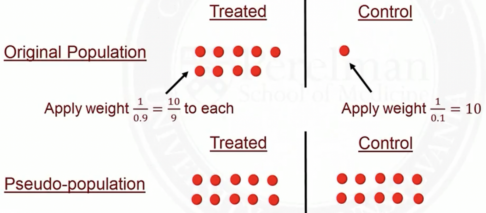
In the original population, some people were more likely to get treated based on their \(X\)’s
In the pseudo-population, everyone is equally likely to get treated, regardless of their \(X\)’s
Estimation with IPTW
We can estimate \(E(Y^1)\) as below \[ \frac{\sum_{i=1}^n \frac{1}{\pi_i} A_i Y_i} {\sum_{i=1}^n \frac{1}{\pi_i} A_i } \]
- where \(\pi_i = P(A_i=1|X_i)\) is the propensity score
- The numerator is the sum of \(Y\)’s in treated pseudo-population
- The denominator is the number of subjects in treated pseudo-population
We can estimate \(E(Y^0)\) as below \[ \frac{\sum_{i=1}^n \frac{1}{1-\pi_i} (1-A_i) Y_i} {\sum_{i=1}^n \frac{1}{1-\pi_i} (1-A_i) } \]
Average treatment effect: \(E(Y^1) - E(Y^0)\)
Marginal Structural Models
Marginal structural models
Marginal structural models (MSM): a model for the mean of the potential outcomes
Marginal: not conditional on the confounders (population average)
Structural: for potential outcomes, not observed outcomes
Linear MSM and logistic MSM
Linear MSM \[ E(Y^a) = \psi_0 + \psi_1 a, \quad a = 0, 1 \]
- \(E(Y^0) = \psi_0\), \(E(Y^0) = \psi_0 + \psi_1\)
- So the average causal effect \[E(Y^1) - E(Y^0) = \psi_1\]
Logistic MSM \[ logit\{E(Y^a)\} = \psi_0 + \psi_1 a, \quad a = 0, 1 \]
- So the causal odds ratio \[ \frac{\frac{P(Y^1=1)}{1-P(Y^1=1)}}{\frac{P(Y^0=1)}{1-P(Y^0=1)}} = \psi_1 \]
MSM with effect modification
Suppose \(V\) is a variable that modifies the effect of \(A\)
A linear MSM with effect modification \[ E(Y^a \mid V) = \psi_0 + \psi_1 a + \psi_3V + \psi_4 a V, \quad a = 0, 1 \]
- So the average causal effect \[E(Y^1) - E(Y^0) = \psi_1 + \psi_4 V\]
- General MSM
\[
g\{E(Y^a \mid V)\} = h(a, V; \psi)
\]
- \(g()\): link function
- \(h()\): a function specifying parametric from of \(a\) and \(V\) (typically additive, linear)
MSM estimation using pseudo-population
Because of confounding, MSM \[ g\{E(Y^a \mid V)\} = \psi_0 + \psi_1 a \] is difference from GLM (generalized linear model) \[ g\{E(Y_i \mid A_i)\} = \psi_0 + \psi_1 A_i \]
Pseudo-population (obtained from IPTW) is free of confounding
- We therefore estimate MSM by solving GLM with IPTW
MSM estimation steps
Estimate propensity score, using logistic regression
Create weights
- Inverse of propensity score for treated subjects
- Inverse of one minus propensity score for control subjects
Specify the MSM of interest
Use software to fit a weighted generalized linear model
Use asymptotic (sandwich) variance estimator
- This accounts for fact that pseudo-population might be larger than sample size
Bootstrap
We may also use bootstrap to estimate standard error
Bootstrap steps
Randomly sample with replacement from the original sample
Estimate parameters
Repeat steps 1 and 2 many times
Use the standard deviation of the bootstrap estimates as an estimate of the standard error
Assessing covariate balance with weights
Covariate balance check with standardized differences
Covariate balance: can be checked on the weighted sample using standardized difference \[ smd = \frac{\bar{X}_{\text{treatment}} - \bar{X}_{\text{control}}}{\sqrt{\frac{s^2_{\text{treatment}} + s^2_{\text{control}}}{2}}} \]
- Weighted means \(\bar{X}_{\text{treatment}}\), \(\bar{X}_{\text{control}}\)
- Weighted variances \(s^2_{\text{treatment}}\), \(s^2_{\text{control}}\)
Balance check tools
- Table 1
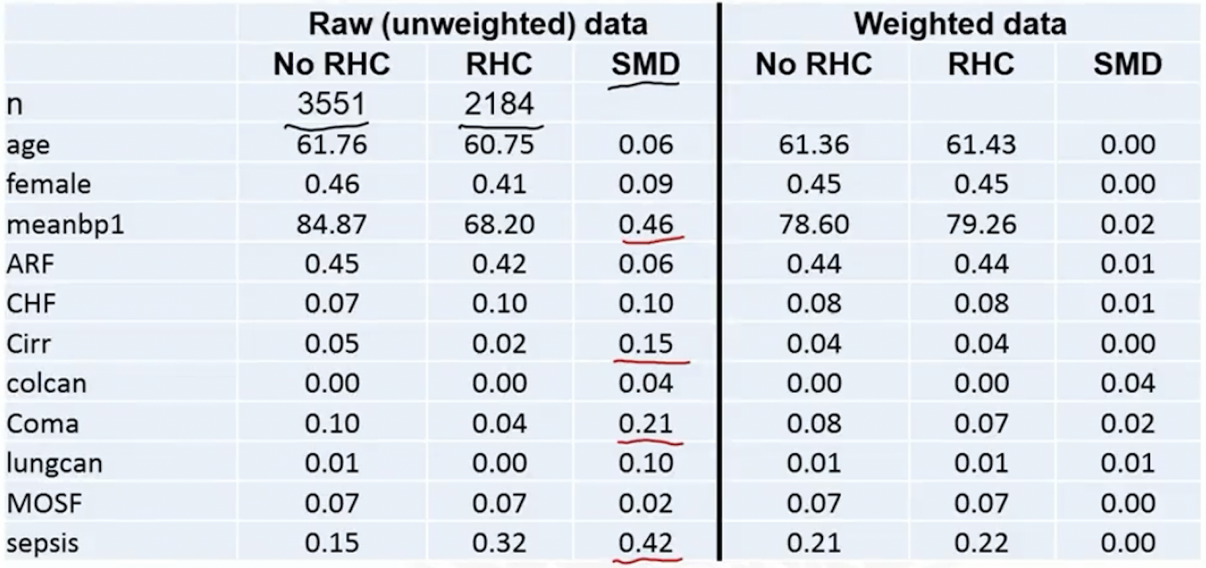
- SMD plot
If imbalance after weighting
Refine propensity score model
- Interactions
- Non-linearity
Then reaccess balance
Problems and remedies for large weights
Larger weights lead to more noise
For an object with a large weight, its outcome data can greatly affect parameter estimation
An object with large weight can also affect standard error estimation, via bootstrap, depending on whether the object is selected or not
An extremely large weights means the probability of that treatment is very small, thus a potential violation of the positivity assumption
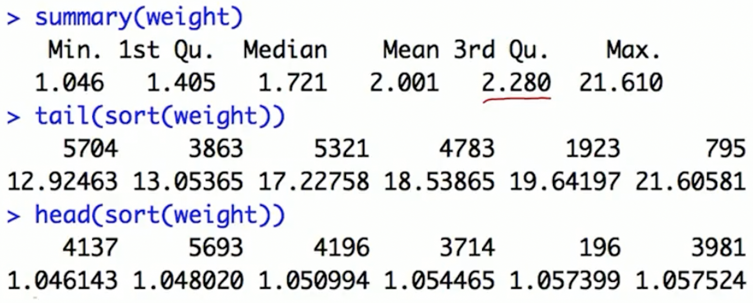
Check weights via plots and summary statistics
- Investigate very large weights: identify the subjects with large weights and find what’s unusual about them
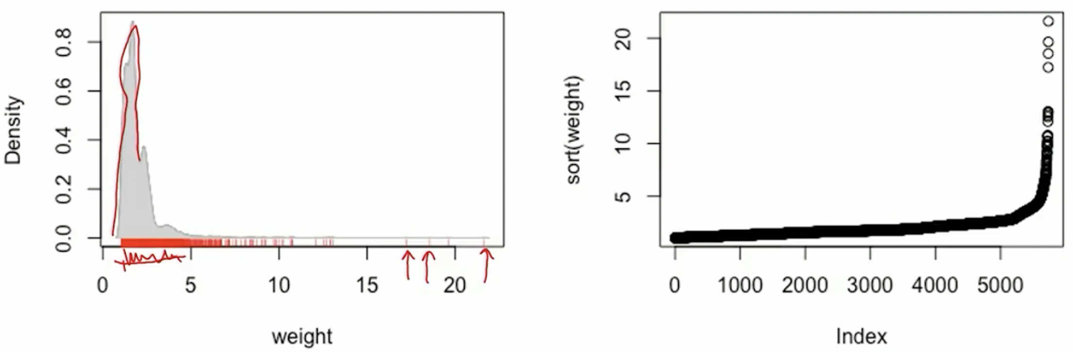
Option 1: trimming the tails
Large weights: occur in the tails of the propensity score distribution
Trim the tails to eliminate some extreme weights
- Remove treated subjects whose propensity scores are above the 98th percentile from the distribution among controls
- Remove control subjects whose propensity scores are below the 2nd percentile from the distribution among treated
Note: trimming the tails changes the population
Option 2: truncating the weights
Another option to deal with large weights is truncation
Weight truncation steps
- Determine a maximum allowable weight
- Can be a specific value (e.g., 100)
- Can based on a percentile (e.g., 99th)
- If a weight is greater than the maximum allowable, set it to the maximum allowable value
- Bias-variance trade-off
- Truncation: bias, but smaller variance
- No truncation: unbiased, larger variance
Truncating extremely large weights can result in estimators with lower MSE
References
Coursera class: “A Crash Course on Causality: Inferring Causal Effects from Observational Data”, by Jason A. Roy (University of Pennsylvania)