State-based vs variable-based search problems: order
There is usually an (obvious) order for state-based search problems, e.g., certain start and end points.
For variable-based search problems:
- Ordering doesn’t affect correctness (e.g., map coloring problem), so we might dynamically choose a better ordering of the variables (e.g., lookahead).
- Variables are interdependent in a local way.
Equivalent terminologies
- Variable-based models \(=\) graphical models
- Probablistic graphical models = \(\{\)Markov networks, Bayesian networks\(\}\)
- Markov networks \(=\) undirected graphical models
- Bayesian networks \(=\) directed graphical models
Constraint Satisfaction Problems (CSPs)
Factor Graphs
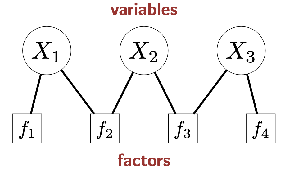
Figure source: Stanford CS221 spring 2025, lecture slides week 6
Variables (and their domains): \[ X = (X_1, \ldots, X_n), \text{ where } X_i \in \text{Domain}_i \]
Factors: constraints or preferrence \[ f_1, \ldots, f_m, \text{ where } f_j(X) \geq 0 \]
- Factors measure how good an assignment is. We prefer \(X\) that can achieve higher value of \(f_j\).
- If \(f_j(X) = 0 \text{ or } 1\), it describes a constraint.
- For example, a factor for force \(X_1\) and \(X_2\) to be equal can be written as \(\mathbf{1}[X_1 = X_2]\).
- Scope of a factor: set of variables it depends on.
- Arity of a factor: number of variables in the scope
- Unary factor: arity 1
- Binary factor: arity 2
Assignment weights: each assignment \(x = (x_1, \ldots, x_n)\) has a weight \[\text{Weight}(x) = \prod_{j=1}^m f_j (x)\]
- An assignment \(x\) is consistent if Weight\((x) > 0\)
Goal: find the best assignment of values to the variables to maximize the weight \[ \arg\max_x \text{Weight}(x) \]
- A CSP is satisfiable if \(\max_x \text{Weight}(x) > 0\).
Exact Backtracking Search
- In backtracking search
- Each node is a partial assignment, and each child node is an extension of the partial assignment.
- Each leaf node is a complete assignment.
- For a partial assignment \(x\) and a new variable \(X_i\) that’s not in \(x\), dependent factor \(D(x, X_i)\) is the set of factors that only depend on \(x\) and \(X_i\), but not on any other variables.
Backtracking search algorithm for CSPs
Backtrack(\(x\), \(w\), Domains):
- If \(x\) is complete assignment: update best and return
- Choose unassigned variable \(X_i\) (MCV)
- Order values in Domain\(_i\) of chosen variable \(X_i\) (LCV)
- For each value \(v\) in that order:
- \(\delta \leftarrow \prod_{f_j \in D(x, X_i)} f_j\left(x \cup \{X_i: v\}\right)\)
- If \(\delta=0\): continue (new partial assignment is inconsistent)
- Domains\(^\prime \leftarrow\) Domains via lookahead
- If any Domains\(^\prime_i\) is empty: continue
- Backtrack(\(x \cup \{X_i: v\}\), \(w\delta\), Domains\(^\prime\))
In the above algorithm, the blue contents are the ones that can be optimized
One-step lookahead: forward checking. After assigning a variable \(X_i\), eliminate inconsistent values from the dominas of \(X_i\)’s neighbors
Dynamic ordering
- Choose an unassigned variable: choose the most constrained variable (MCV), i.e., the variable that has the smallest domain).
- If going to fail, fail early (more pruning)
- Because we need to find an assignment for every variable
- This is useful when some factor are constraints (can prune assginemnts with weight 0)
- Order values of a selected variable: least constrained value (LCV), descending order of the sum of consistent values of neighboring variables
- Choose value that is most likely to lead to solution
- Because for each variable only need to choose some values
- Useful when all factors are constraints (Only need to find an assignment with weight 1)
Arc consistency
A variable \(X_i\) is arc consistent wrt \(X_j\) if for each \(x_i \in \text{Domain}_i\), there exists \(x_j \in \text{Domain}_j\) such that \[ f(\{X_i: x_i, X_j: x_j \}) \neq 0 \] for all factors \(f\) whose scope contains \(X_i\) and \(X_j\).
AC-3 algorithm: repeatedly enforce arc consistency on all variables
Approximate Search
- Backtracking and beam search: extend partial assignments
- Local search: modify complete assignments
Beam search
- Greedy search: we assume we have a fixed ordering of the variables. Then in every step of assigning a value to a variable, greedy search is to use the assignment with the highest weight
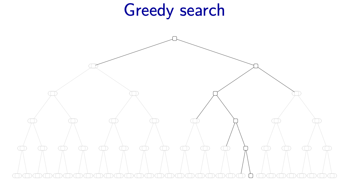
Figure source: Stanford CS221 spring 2025, lecture slides week 6
- Beam search: keep track of (at most) \(K\) best partial assignments at each level of the search tree
- Note: these candidates are not guaranteed to be the \(K\) best at each level
- Time complexity of beam search is \(O(nKb)\)
- Depth: number of variables \(n\)
- Branching factor \(b = |\text{Domain}_i|\)
- Beam size \(K\)
- Beam size \(K\) controls trade-off between efficiency and accuracy
- \(K=1\): greedy search, \(O(nb)\) time
- \(K = \infty\): BFS, \(O(b^n)\) time
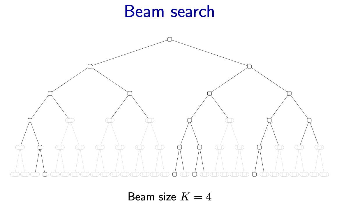
Figure source: Stanford CS221 spring 2025, lecture slides week 6
Local search
The goal is to improve an old complete assignment.
Locality: When evaluating possible re-assignments to \(X_i\), only need to consider the factors that depend on \(X_i\).
Iterated conditional modes (ICM) algorithm
- Initialize \(x\) to a random complete assignment
- Loop through \(i = 1, \ldots, n\) until convergence:
- Compute weight of \(x_v = x\cup \{X_i: v\}\) for each \(v\)
- \(x \leftarrow x_v\) with highest weights
ICM can stuck at local optima
ICM has linear time complexity
Markov Networks
A Markov network is a factor graph which defines a joint distribution over random variables \(X = (X_1, \ldots, X_n)\): \[ \mathbb{P}(X = x) = \frac{\text{Weight}(x)}{Z} \] where \(Z = \sum_{x^\prime} \text{Weight}(x^\prime)\) is the normalization constant.
- Markov network \(=\) factor graphs \(+\) probability
Marginal probability of \(X_i = v\) is \[ \mathbb{P}(X_i = v) = \sum_{x: x_i = v} \mathbb{P}(X = x) \]
Gibbs Sampling
- Gibbs sampling algorithm:
- Initialize \(x\) to a random complete assignment
- Loop through \(i = 1, \ldots, n\) until convergence:
- Set \(x_i = v\) with probability \[\mathbb{P}(X_i = v \mid X_{-i} = x_{-i})\]
- Increment count\(_i(x_i)\)
- Estimate \[\hat{\mathbb{P}}(X_i = x_i) = \frac{\text{count}_i (x_i)}{\sum_v \text{count}_i (v)}\]
- Search vs sampling
| Iterated Conditional Modes | Gibbs Sampling |
|---|---|
| maximum weight assignment | marginal probabilities |
| choose best value | sample a value |
| converges to local optimum | marginals converge to correct answer |
Bayesian Networks
- Markov networks vs Bayesian networks
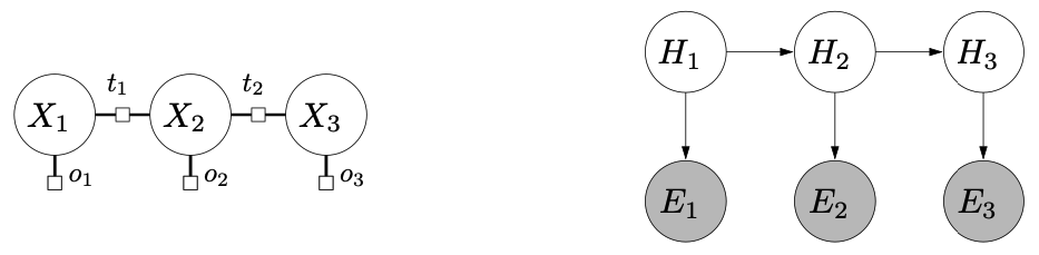
Figure source: Stanford CS221 spring 2025, lecture slides week 7
| Markov networks | Bayesian networks |
|---|---|
| arbitrary factors | local conditional probabilities |
| set of preferences | generative process |
| un-directed graphs | directed graphs |
Let \(X = (X_1, \ldots, X_n)\) be random variables. A Bayesian network is a directed acyclic graph (DAG) that specifies a joint distribution over \(X\) as a project of local conditional distributions, one for each node \[ \mathbb{P}(X_1 =x_1, \ldots, X_n = x_n) \stackrel{\text{def}}{=} \prod_{i=1}^n p\left(x_i \mid x_{\text{Parents}(i)} \right) \]
Reducing Bayesian networks to Markov networks
- Remember to have a single factor connecting each parent.
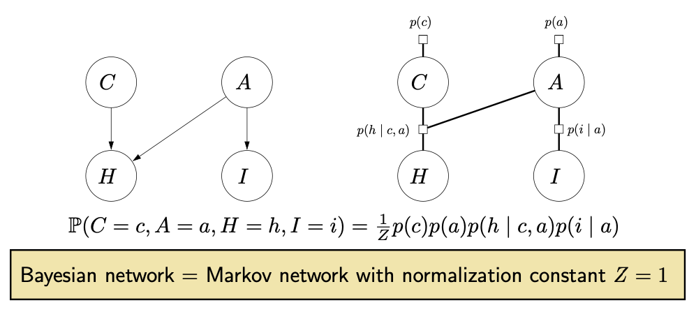
Figure source: Stanford CS221 spring 2025, lecture slides week 7
- Leveraging additional structure
- Throw away any unobserved leaves before running inference
- Throw away any disconnected components before running inference (independence)
Parameter Estimation
Smoothing
- Laplace smoothing: for each distribution \(d\) and partial assignment \((x_{\text{Parents}(i)}, x_i)\), add \(\lambda\) to count\(_d(x_{\text{Parents}(i)}, x_i)\)
- This is like adding a Dirichlet prior
Expectation Maximization (EM) Algorithm
- Initialize \(\theta\) randomly
- Repeat until converge
- E step: fix \(\theta\), update \(H\)
- For each \(h\) compute \[q(h) = \mathbb{P}(H=h \mid E=e, \theta)\]
- Create fully-observed weighted examples: \((h, e)\) with weight \(q(h)\)
- M step: fix \(H\), update \(\theta\)
- Maximum likelihood (count and normalize) on weighted examples to get \(\theta\)
- E step: fix \(\theta\), update \(H\)
- Properties of the EM algorithm
- EM algorithm deals with hidden variables \(H\)
- Intuition: generalization of the K-means algorithm:
- Cluster centroids = parameter \(\theta\)
- Cluster assignments = hidden variables \(H\)
- EM algorithm converges to local optima
A more general version of the EM algorithm
Choose the initial parameters \(\boldsymbol\theta^{\text{old}}\)
E step: since the conditional posterior \(p\left( \mathbf{Z} \mid \mathbf{X}, \boldsymbol\theta^{\text{old}} \right)\) contains all of our knowledge about the latent variable \(\mathbf{Z}\), we compute the expected complete-data log likelihood under it. \[\begin{align*} \mathcal{Q}(\boldsymbol\theta, \boldsymbol\theta^{\text{old}}) & = E_{\mathbf{Z} \mid \mathbf{X}, \boldsymbol\theta^{\text{old}}} \left\{\log p(\mathbf{X}, \mathbf{Z} \mid \boldsymbol\theta) \right\} \\ & = \sum_{\mathbf{Z}} p\left( \mathbf{Z} \mid \mathbf{X}, \boldsymbol\theta^{\text{old}} \right) \log p(\mathbf{X}, \mathbf{Z} \mid \boldsymbol\theta) \end{align*}\]
M step: revise parameter estimate \[ \boldsymbol\theta^{\text{new}} = \arg\max_{\boldsymbol\theta} \mathcal{Q}(\boldsymbol\theta, \boldsymbol\theta^{\text{old}}) \]
- Note in the maximizing step, the logarithm acts driectly on the joint likelihood \(p(\mathbf{X}, \mathbf{Z} \mid \boldsymbol\theta)\), so the maximizating will be tractable.
Check for convergence of the log likelihood or the parameter values. If not converged, use \(\boldsymbol\theta^{\text{new}}\) to replace \(\boldsymbol\theta^{\text{old}}\), and return to step 2.
See my EM algorithm notes for more details